Parallel Resonance Circuit

Parallel Resonance Circuit: Tank Circuits and Anti-Resonance

Introduction to Parallel Resonance

While series resonance circuits are characterized by minimum impedance and maximum current, Parallel Resonance Circuits exhibit the opposite behavior: maximum impedance and minimum current at the resonant frequency. This unique characteristic makes parallel resonance circuits invaluable as “rejector circuits” that block or reject specific frequencies while allowing others to pass.

Also known as anti-resonance or tank circuits, parallel resonance configurations are fundamental building blocks in radio frequency (RF) oscillators, band-stop filters, impedance matching networks, and tuned amplifiers. Understanding the differences between series and parallel resonance is crucial for designing efficient filters, oscillators, and communication systems.

In a parallel resonance circuit, the inductor and capacitor are connected in parallel across an AC voltage source, often with a resistor representing either the coil’s internal resistance or a separate parallel resistance. At resonance, the reactive currents in the inductor and capacitor branches cancel each other, leaving only a small resistive current drawn from the source.

This comprehensive guide will explore the physics, mathematics, and practical applications of parallel resonance circuits, complete with visual diagrams and step-by-step calculations.

What is Parallel Resonance?
Parallel resonance occurs when an inductor and capacitor are connected in parallel and their reactances are equal (X_L = X_C). At this resonant frequency, the circuit exhibits maximum impedance and minimum current draw from the source. Unlike series resonance which maximizes current, parallel resonance minimizes it, making it ideal for rejector circuits and oscillators.

The Physics of Parallel Resonance

Circuit Configuration

A practical parallel resonance circuit typically consists of:

• An inductor (L) with its internal resistance (R_L) in series
• A capacitor (C) connected in parallel with the inductor
• Sometimes an additional parallel resistance (R_p) representing load or losses

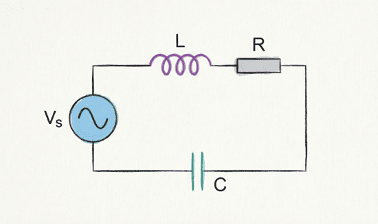
The key difference from series resonance is that in parallel configuration, the voltage is the same across both the inductor and capacitor branches, but the currents are different and can be much larger than the source current.

Current Circulation and Tank Action

At resonance, something fascinating happens: while the total current drawn from the source is minimum, large currents circulate between the inductor and capacitor. Energy oscillates back and forth between the magnetic field of the inductor and the electric field of the capacitor, much like water sloshing back and forth in a tank—hence the name “tank circuit.”

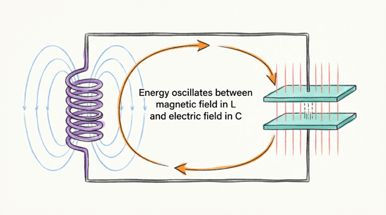
The circulating current can be Q times larger than the source current, where Q is the quality factor. This internal current circulation is what gives the tank circuit its energy storage capability.

The Resonant Frequency

For an ideal parallel LC circuit (ignoring resistance), the resonant frequency formula is identical to series resonance:

$f_r = \frac{1}{2\pi\sqrt{LC}}$

However, in practical circuits where the inductor has significant resistance, the resonant frequency is slightly modified:

$f_r = \frac{1}{2\pi\sqrt{LC}} \sqrt{1 – \frac{R^2 C}{L}}$

For most practical applications where R is small compared to X_L, this simplifies to the ideal formula.

What is the resonant frequency formula for parallel resonance?
The resonant frequency for parallel resonance is f_r = 1/(2π√LC), identical to series resonance. However, practical parallel circuits with significant resistance have a slightly lower resonant frequency due to the resistive effects.

Characteristics of Parallel Resonance

1. Maximum Impedance

At resonance, the parallel LC combination presents maximum impedance to the source. This is the opposite of series resonance. The impedance at resonance can be calculated as:

$Z_{max} = \frac{L}{RC}$ (for practical parallel circuits)

Or, in terms of Q factor:

$Z_{max} = Q^2 \times R$

Where R is the series resistance of the coil. This high impedance at resonance is why parallel resonance circuits are called “rejector circuits”—they reject current flow at the resonant frequency.

2. Minimum Current

Since impedance is maximum at resonance, the total current drawn from the source reaches its minimum value:

$I_{min} = \frac{V}{Z_{max}}$

This is significantly lower than the current at frequencies above or below resonance. The circuit draws very little power from the source at resonance, making it highly efficient for oscillator applications.

3. Unity Power Factor

At resonance, the circuit behaves as a purely resistive load:

• The reactive components cancel in the admittance domain
• Voltage and total current are in phase
• Power factor = 1.0 (unity)
• The circuit draws only real power (minimal) from the source

4. Current Magnification

While the source current is minimum at resonance, the branch currents (current through L and C individually) can be very large:

$I_L = I_C = Q \times I_{source}$

This current magnification is analogous to voltage magnification in series resonance. The circulating current between L and C can be many times larger than the current supplied by the source.

5. Dynamic Impedance

The impedance at resonance is sometimes called dynamic impedance or dynamic resistance because it represents the effective resistance of the tank circuit at the resonant frequency. For high-Q circuits, this can be tens or hundreds of kilohms, even though the coil’s DC resistance might be only a few ohms.

Visualizing Parallel Resonance

Admittance and Impedance vs. Frequency

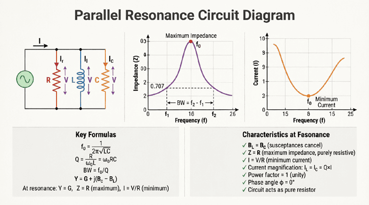
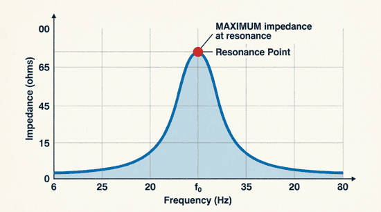
The admittance (Y = 1/Z) of a parallel RLC circuit is minimum at resonance, which means impedance is maximum. The impedance curve shows:

• Below resonance (f < f_r): Capacitive branch dominates, impedance is lower and capacitive
• At resonance (f = f_r): Reactances cancel, impedance is maximum
• Above resonance (f > f_r): Inductive branch dominates, impedance is lower and inductive

Current vs. Frequency Curve

The total current drawn from the source is the inverse of the impedance:

• At resonance: Current is minimum
• Away from resonance: Current increases as impedance decreases

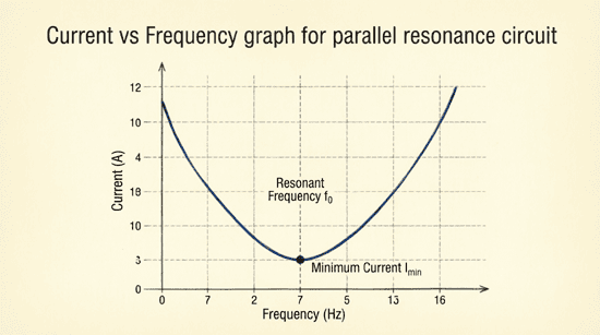
The sharpness of the current minimum (or impedance maximum) depends on the circuit’s Q factor.

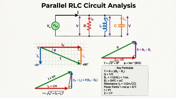
Phasor Diagram at Resonance

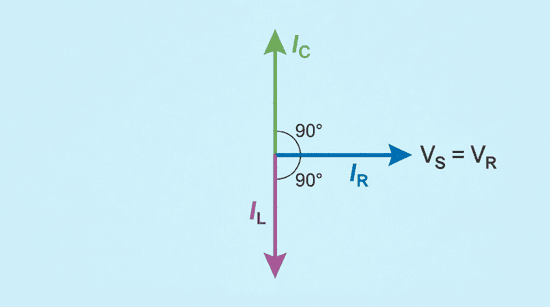
At resonance, the phasor diagram shows:

• $I_R$ is horizontal (in phase with voltage)
• $I_L$ points down (lagging voltage by 90°)
• $I_C$ points up (leading voltage by 90°)
• $I_L$ and $I_C$ are equal in magnitude and opposite in direction
• The source current $I_S$ equals $I_R$ (since $I_L$ and $I_C$ cancel)

Quality Factor (Q Factor) and Bandwidth

The Quality Factor for Parallel Resonance

For parallel resonance, the Q factor is defined as the ratio of the circulating current to the source current, or equivalently:

$Q = \frac{R_p}{X_L} = \frac{R_p}{X_C} = R_p \sqrt{\frac{C}{L}}$

Where $R_p$ is the equivalent parallel resistance.

Alternatively, if the inductor has series resistance $R_s$:

$Q = \frac{X_L}{R_s} = \frac{\omega_r L}{R_s}$

This is the same formula as for series resonance, but the interpretation differs.

Bandwidth for Parallel Resonance

The bandwidth formula is identical to series resonance:

$BW = f_2 – f_1 = \frac{f_r}{Q}$

Where:

• $f_2$ = Upper cutoff frequency (higher -3dB point)
• $f_1$ = Lower cutoff frequency (lower -3dB point)
• $f_r$ = Resonant frequency
• $Q$ = Quality factor

At the half-power frequencies (cutoff frequencies):

• Impedance = $0.707 \times Z_{max}$
• Current = $\sqrt{2} \times I_{min}$
• The circuit impedance drops to 70.7% of its maximum value

Selectivity

• High Q (> 10): Narrow bandwidth, sharp impedance peak, highly selective. Used in radio tuners and narrowband filters.
• Low Q (< 10): Wide bandwidth, broad impedance curve, less selective. Used in wideband applications.

How does parallel resonance differ from series resonance?
Parallel resonance exhibits maximum impedance and minimum current at resonance, while series resonance has minimum impedance and maximum current. Parallel circuits act as rejector circuits (blocking resonant frequency), while series circuits act as acceptor circuits (passing resonant frequency). Both have the same resonant frequency formula: f_r = 1/(2π√LC).

Step-by-Step Practical Example

Let’s analyze a complete parallel resonance circuit.

Problem Statement:
A parallel resonance circuit has the following components:

• Inductor: $L = 50 \text{ mH} = 0.05 \text{ H}$ with internal resistance $R = 10 \Omega$
• Capacitor: $C = 20 \text{ nF} = 20 \times 10^{-9} \text{ F}$
• Supply voltage: $V = 50\text{V (RMS)}$

Calculate:

1. Resonant frequency ($f_r$)
2. Inductive and capacitive reactance at resonance
3. Quality factor (Q)
4. Dynamic impedance at resonance ($Z_{max}$)
5. Total current at resonance ($I_{min}$)
6. Circulating current in L and C branches
7. Bandwidth (BW)
8. Lower and upper cutoff frequencies ($f_1$ and $f_2$)

Solution:

Step 1: Calculate Resonant Frequency

$f_r = \frac{1}{2\pi\sqrt{LC}}$

$f_r = \frac{1}{2\pi\sqrt{0.05 \times 20 \times 10^{-9}}}$

$f_r = \frac{1}{2\pi\sqrt{1 \times 10^{-9}}}$

$f_r = \frac{1}{2\pi \times 3.162 \times 10^{-5}}$

$f_r = \frac{1}{1.987 \times 10^{-4}}$

$f_r \approx 5033 \text{ Hz} = 5.033 \text{ kHz}$

Step 2: Calculate Reactances at Resonance

$X_L = 2\pi f_r L = 2\pi \times 5033 \times 0.05$

$X_L \approx 1581 \Omega$

At resonance, $X_C = X_L$:

$X_C \approx 1581 \Omega$

Step 3: Calculate Quality Factor

$Q = \frac{X_L}{R} = \frac{1581\Omega}{10\Omega}$

$Q \approx 158.1$

This is a very high-Q circuit, indicating sharp selectivity.

Step 4: Calculate Dynamic Impedance at Resonance

$Z_{max} = \frac{L}{RC} = \frac{0.05}{10 \times 20 \times 10^{-9}}$

$Z_{max} = \frac{0.05}{2 \times 10^{-7}}$

$Z_{max} = 250,000 \Omega = 250 \text{ k}\Omega$

Alternatively: $Z_{max} = Q^2 \times R = (158.1)^2 \times 10 \approx 250 \text{ k}\Omega$

Step 5: Calculate Total Current at Resonance

$I_{min} = \frac{V}{Z_{max}} = \frac{50\text{V}}{250,000\Omega}$

$I_{min} = 0.0002 \text{ A} = 0.2 \text{ mA}$

Step 6: Calculate Circulating Branch Currents

Current through inductor:
$I_L = \frac{V}{X_L} = \frac{50\text{V}}{1581\Omega}$

$I_L \approx 0.0316 \text{ A} = 31.6 \text{ mA}$

Current through capacitor:
$I_C = \frac{V}{X_C} = \frac{50\text{V}}{1581\Omega}$

$I_C \approx 0.0316 \text{ A} = 31.6 \text{ mA}$

Notice: The circulating currents (31.6 mA) are much larger than the source current (0.2 mA)!

Current magnification ratio: $31.6 \text{ mA} / 0.2 \text{ mA} = 158$, which equals Q!

Step 7: Calculate Bandwidth

$BW = \frac{f_r}{Q} = \frac{5033}{158.1}$

$BW \approx 31.8 \text{ Hz}$

This is a very narrow bandwidth, confirming high selectivity.

Step 8: Calculate Cutoff Frequencies

$f_1 = f_r – \frac{BW}{2} = 5033 – \frac{31.8}{2}$

$f_1 \approx 5017 \text{ Hz}$

$f_2 = f_r + \frac{BW}{2} = 5033 + \frac{31.8}{2}$

$f_2 \approx 5049 \text{ Hz}$

The circuit passes frequencies between 5017 Hz and 5049 Hz with high impedance, rejecting the resonant frequency of 5033 Hz.

Practical Applications of Parallel Resonance

1. RF Oscillators and Tank Circuits

Parallel resonance circuits are the heart of RF oscillators used in radio transmitters, signal generators, and clock circuits. The tank circuit stores energy and oscillates at its natural resonant frequency. When combined with an active device (transistor or op-amp) to compensate for losses, it produces a stable sinusoidal output at $f_r$.

2. Band-Stop (Notch) Filters

Parallel resonance circuits are used as notch filters to eliminate specific unwanted frequencies. For example:

• Removing 60 Hz power line hum from audio signals
• Eliminating interference at specific frequencies in communication systems
• Filtering out harmonics in power systems

At resonance, the high impedance blocks the unwanted frequency from passing through.

3. Impedance Matching Networks

In RF amplifiers and antenna systems, parallel resonance circuits are used to transform impedances, ensuring maximum power transfer between stages with different impedance levels.

4. Tuned Amplifiers

Radio and TV receivers use parallel resonance circuits as load impedances in amplifier stages. The amplifier provides high gain only at the resonant frequency, effectively selecting the desired station while rejecting others.

5. Induction Heating (Parallel Configuration)

Some induction heating systems use parallel resonance to create high voltages across the work coil, which then produces the high currents needed for heating.

6. Power Factor Correction

While series capacitors are sometimes used, parallel capacitors are more commonly used for power factor correction in industrial facilities. The capacitor bank is tuned to avoid resonance with system inductance at harmonic frequencies.

Comparison: Series vs. Parallel Resonance

Characteristic	Series Resonance	Parallel Resonance
Impedance at $f_r$	Minimum (= R)	Maximum (= L/RC)
Current at $f_r$	Maximum	Minimum
Circuit Type	Acceptor circuit	Rejector circuit
Magnification	Voltage magnification	Current magnification
Power Factor	Unity (1.0)	Unity (1.0)
Applications	Band-pass filters, tuners	Band-stop filters, oscillators
Branch Currents	Same as source	Q × source current
Component Voltages	Q × source voltage	Same as source voltage

Conclusion

Parallel resonance circuits represent a fundamental concept in AC circuit theory with unique characteristics that complement series resonance. The ability to create maximum impedance and minimum current at a specific frequency makes parallel resonance indispensable in oscillator design, filtering applications, and impedance matching networks.

Key takeaways from this guide include:

1. Resonant Frequency: $f_r = 1/(2\pi\sqrt{LC})$ – identical to series resonance
2. Maximum Impedance: At resonance, $Z_{max} = L/(RC) = Q^2 \times R$
3. Minimum Current: $I_{min} = V/Z_{max}$ at resonance
4. Current Magnification: Branch currents = Q × source current
5. Quality Factor: $Q = X_L/R = \omega_r L/R$ – determines selectivity
6. Bandwidth: $BW = f_r/Q$ – narrower for higher Q
7. Tank Action: Energy circulates between L and C with minimal source current

Understanding parallel resonance equips you to design stable oscillators, effective notch filters, and efficient impedance matching networks. Whether you’re building a radio transmitter, eliminating interference, or designing a precision filter, the principles of parallel resonance are essential tools in your electrical engineering arsenal.