Parallel RLC Circuit Analysis

July 12, 2026 Creatives AD

Parallel RLC Circuit Analysis: The Complete Guide to AC Networks

In our previous exploration of the series RLC circuit, we discovered how components behave when connected end-to-end in a single path. We learned that in a series circuit, the current is the same everywhere, making it our reference point for analysis. However, electrical engineering offers another fundamental configuration: the Parallel RLC Circuit.

In a parallel RLC circuit, the resistor (R), inductor (L), and capacitor (C) are connected across the same two nodes, creating multiple separate paths (branches) for the current to flow from the AC voltage source. This configuration fundamentally shifts our analytical perspective. Instead of dealing with a single, constant current and varying voltages, we now have a single, constant voltage and varying branch currents.

Analyzing a parallel RLC circuit requires us to apply the principles of phasor addition to currents rather than voltages. We must calculate how the inductive and capacitive branch currents interact, determine the total current drawn from the source, and understand how this configuration impacts the overall impedance and power factor of the system. This comprehensive guide will walk you through the step-by-step analysis of the parallel RLC circuit, completing your mastery of fundamental AC network theory.

What is a Parallel RLC Circuit?
A parallel RLC circuit is an AC electrical circuit where a resistor, an inductor, and a capacitor are connected in parallel across a common AC voltage source. In this configuration, the exact same voltage is applied across all three components, but the current flowing through each individual branch will differ in both magnitude and phase angle.

The Golden Rule of Parallel Circuits: Voltage is the Reference

Before we begin calculating currents and impedance, we must establish the foundational rule of parallel circuit analysis: In a parallel circuit, the voltage is the same across all branches.

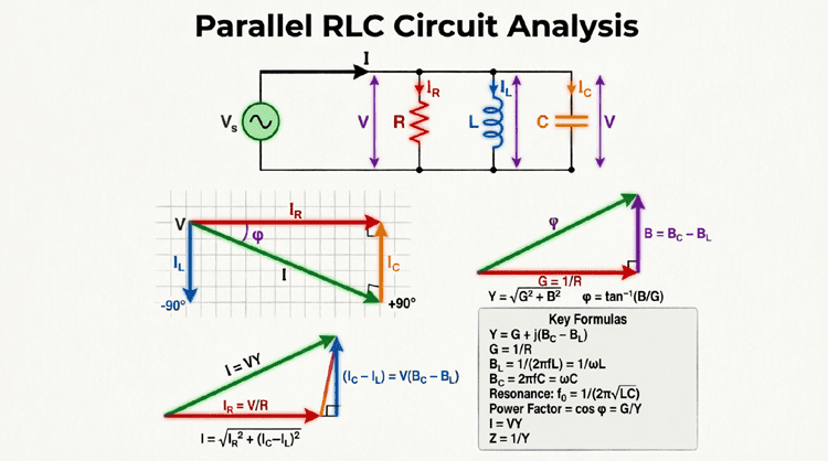
Because the exact same alternating voltage is applied simultaneously to the resistor, the inductor, and the capacitor, it is highly convenient to use the voltage phasor ($V$) as our reference vector. We draw the voltage phasor horizontally along the 0° axis. All branch currents are then drawn and calculated relative to this reference voltage.

Branch Currents and Phase Relationships

Based on the individual characteristics of R, L, and C, we know exactly how their respective branch currents relate to the reference voltage:

Resistor Current ($I_R$): In a resistor, voltage and current are in phase. Therefore, the $I_R$ phasor points in the exact same direction as the voltage reference (0°).
Inductor Current ($I_L$): In an inductor, current lags voltage by 90°. Therefore, the $I_L$ phasor points straight down along the negative imaginary (-j) axis.
Capacitor Current ($I_C$): In a capacitor, current leads voltage by 90°. Therefore, the $I_C$ phasor points straight up along the positive imaginary (+j) axis.

Because $I_L$ and $I_C$ point in directly opposite directions on the complex plane, they inherently oppose each other. The net reactive current is simply the difference between the two: $I_X = I_C – I_L$ (or $I_L – I_C$, depending on which is larger).

Calculating Branch Currents

The first step in analyzing a parallel RLC circuit is to calculate the current flowing through each individual branch. Since the voltage ($V$) is known and constant across all branches, we simply apply the AC version of Ohm’s Law ($I = V / Z$) to each component individually.

The Formulas

Resistive Branch Current: $I_R = \frac{V}{R}$
Inductive Branch Current: $I_L = \frac{V}{X_L}$
Capacitive Branch Current: $I_C = \frac{V}{X_C}$

These calculations yield the RMS magnitude of the current in each branch. Because we are using the voltage as our 0° reference, we can also assign phase angles to these currents:

$I_R$ is at $0^\circ$
$I_L$ is at $-90^\circ$
$I_C$ is at $+90^\circ$

Calculating Total Current: The Current Triangle

Once we have the individual branch currents, we must find the total current ($I_{total}$) drawn from the AC source. Because these currents are not in phase with each other, we cannot simply add them together using standard arithmetic ($I_{total} \neq I_R + I_L + I_C$). Instead, we must add them as phasors (vectors).

The Net Reactive Current

Since the inductive current ($I_L$) and capacitive current ($I_C$) are 180 degrees out of phase with each other, they subtract. The net reactive current ($I_X$) is:

$I_X = I_C – I_L$ (or mathematically, the absolute difference $|I_L – I_C|$)

If $I_L > I_C$, the net reactive current is inductive (points down, lagging).
If $I_C > I_L$, the net reactive current is capacitive (points up, leading).

The Total Current Formula

Because the resistive current ($I_R$) and the net reactive current ($I_X$) are 90 degrees out of phase, we use the Pythagorean theorem to find the magnitude of the total current:

$I_{total} = \sqrt{I_R^2 + (I_C – I_L)^2}$

The Current Triangle

The relationship between $I_R$, $I_X$, and $I_{total}$ is beautifully visualized using the Current Triangle. Notice how this is the exact dual of the Impedance Triangle used in series circuits.

Diagram Description: The Soft Sky Blue horizontal line represents the Resistive Current ($I_R$). The Soft Teal vertical line represents the Net Capacitive Current ($I_C – I_L$). The Soft Green diagonal line represents the Total Current ($I_{total}$). The angle θ between $I_R$ and $I_{total}$ is the circuit’s phase angle. (Note: If the circuit were net inductive, the vertical line would point downward).

Phase Angle and Power Factor

The phase angle ($\theta$) of a parallel RLC circuit tells us the exact degree by which the total current lags or leads the source voltage. It is calculated using the trigonometric tangent function based on the current triangle:

$\theta = \arctan\left(\frac{I_C – I_L}{I_R}\right)$

Note: If $I_L$ is greater than $I_C$, the formula is often written as $\arctan((I_L – I_C) / I_R)$ to yield a positive angle representing a lag.

The phase angle is directly tied to the Power Factor (PF) of the circuit:

Power Factor = $\cos(\theta) = \frac{I_R}{I_{total}}$

A negative $\theta$ (or $I_L > I_C$) indicates a lagging power factor (inductive dominance).
A positive $\theta$ (or $I_C > I_L$) indicates a leading power factor (capacitive dominance).

How do you calculate total current in a parallel RLC circuit?
To calculate total current in a parallel RLC circuit, first find the individual branch currents ($I_R = V/R$, $I_L = V/X_L$, $I_C = V/X_C$). Then, subtract the inductive current from the capacitive current to find the net reactive current. Finally, use the Pythagorean theorem: $I_{total} = \sqrt{I_R^2 + (I_C – I_L)^2}$.

Alternative Method: Admittance, Conductance, and Susceptance

While the current triangle is highly intuitive, advanced AC analysis often uses the concept of Admittance ($Y$) for parallel circuits. Admittance is the reciprocal of impedance ($Y = 1/Z$) and represents how easily a circuit allows current to flow. It is measured in Siemens (S).

In a parallel RLC circuit, total admittance is the phasor sum of its components:

Conductance ($G$): The reciprocal of resistance ($G = 1/R$). Measured in Siemens.
Inductive Susceptance ($B_L$): The reciprocal of inductive reactance ($B_L = 1/X_L$).
Capacitive Susceptance ($B_C$): The reciprocal of capacitive reactance ($B_C = 1/X_C$).

The total admittance is calculated as:
$Y_{total} = \sqrt{G^2 + (B_C – B_L)^2}$

Once $Y_{total}$ is found, the total impedance is simply $Z = 1 / Y_{total}$, and the total current is $I_{total} = V \times Y_{total}$. This method is mathematically elegant and scales easily to parallel circuits with many complex branches.

Step-by-Step Practical Example

Let’s put theory into practice with a complete, step-by-step analysis of a parallel RLC circuit.

Problem Statement:
A parallel RLC circuit is connected to a 120V (RMS), 60Hz AC source. The circuit contains:

A Resistor: $R = 40 \Omega$
An Inductor with an inductive reactance: $X_L = 30 \Omega$
A Capacitor with a capacitive reactance: $X_C = 60 \Omega$

Calculate the branch currents, total current, total impedance, and the phase angle.

Step 1: Calculate Branch Currents

Using Ohm’s Law for each branch ($I = V / Z$):

Resistive Current ($I_R$):
$I_R = \frac{120\text{V}}{40 \Omega} = \mathbf{3.0 \text{ A}}$ (In phase with V, 0°)
Inductive Current ($I_L$):
$I_L = \frac{120\text{V}}{30 \Omega} = \mathbf{4.0 \text{ A}}$ (Lags V by 90°, -90°)
Capacitive Current ($I_C$):
$I_C = \frac{120\text{V}}{60 \Omega} = \mathbf{2.0 \text{ A}}$ (Leads V by 90°, +90°)

Step 2: Calculate Net Reactive Current and Total Current

First, find the net reactive current ($I_X$). Since $I_L$ (4.0A) is greater than $I_C$ (2.0A), the circuit is net inductive.
$I_X = I_L – I_C = 4.0 \text{A} – 2.0 \text{A} = \mathbf{2.0 \text{ A}}$ (Lagging)

Next, calculate the total current ($I_{total}$) using the Pythagorean theorem:
$I_{total} = \sqrt{I_R^2 + I_X^2}$
$I_{total} = \sqrt{3.0^2 + 2.0^2}$
$I_{total} = \sqrt{9 + 4} = \sqrt{13}$
$I_{total} \approx 3.61 \text{ Amps (RMS)}$

Step 3: Calculate Total Impedance

Now that we know the total voltage and total current, we can find the total equivalent impedance of the parallel network using Ohm’s Law:
$Z_{total} = \frac{V}{I_{total}}$
$Z_{total} = \frac{120\text{V}}{3.61\text{A}}$
$Z_{total} \approx 33.24 \Omega$

Notice that the total impedance (33.24 Ω) is actually lower than the smallest individual branch resistance/reactance (30 Ω). This is a fundamental rule of all parallel circuits: the total equivalent impedance is always less than the smallest individual branch impedance.

Step 4: Calculate the Phase Angle

Finally, we calculate the phase angle ($\theta$) of the total current relative to the voltage:
$\theta = \arctan\left(\frac{I_X}{I_R}\right) = \arctan\left(\frac{2.0}{3.0}\right) = \arctan(0.667)$
$\theta \approx 33.69^\circ$

Because the inductive current was larger than the capacitive current, the total current lags the source voltage by 33.69 degrees. The power factor is $\cos(33.69^\circ) \approx 0.832$ lagging.

Why is total impedance in a parallel circuit always lower than the smallest branch impedance?
In a parallel circuit, adding more branches provides additional paths for current to flow. According to Ohm’s Law, more total current for the same voltage means lower total opposition. Therefore, the total equivalent impedance will always be less than the impedance of the smallest individual branch.

Visualizing the Current Phasor Diagram

To truly understand the relationships in our practical example, we can draw a Current Phasor Diagram. Remember, we use the voltage ($V$) as our horizontal reference (0°).

Diagram Description: The Soft Sky Blue vector represents $I_R$ on the horizontal axis. The Soft Teal vector represents $I_C$ pointing straight up. The Soft Plum vector represents $I_L$ pointing straight down. Because $I_L$ is larger than $I_C$, the net reactive current points down. The Dark Slate vector represents the Total Current ($I_{total}$), connecting the origin to the final tip, lagging the voltage by 33.69 degrees.

Power in a Parallel RLC Circuit

Just like in series circuits, a parallel RLC circuit consumes Real Power, exchanges Reactive Power, and draws Apparent Power. The formulas are conceptually identical, but we use the branch currents and voltages to calculate them.

Real Power (P)

Real power is consumed only by the resistive branch.
$P = V \times I_R$ (or $P = I_R^2 \times R$)
Measured in Watts (W).

Reactive Power (Q)

Reactive power is exchanged by the inductive and capacitive branches. Because they oppose each other, we use the net reactive current.
$Q = V \times I_X$ (where $I_X = |I_L – I_C|$)
Measured in Volt-Amperes Reactive (VAR).

Apparent Power (S)

Apparent power is the total power supplied by the source, calculated using the total voltage and total current.
$S = V \times I_{total}$
Measured in Volt-Amperes (VA).

Let’s calculate the power for our practical example ($V = 120V$, $I_R = 3A$, $I_X = 2A$, $I_{total} = 3.61A$):

Real Power (P): $120 \times 3 = \mathbf{360 \text{ W}}$
Reactive Power (Q): $120 \times 2 = \mathbf{240 \text{ VAR}}$ (Inductive)
Apparent Power (S): $120 \times 3.61 = \mathbf{433.2 \text{ VA}}$

Notice that $S = \sqrt{P^2 + Q^2}$ ($\sqrt{360^2 + 240^2} = 432.6$, with minor rounding differences). The Power Triangle for a parallel circuit is geometrically identical to the Current Triangle, just scaled by the factor of $V$.

Practical Applications of Parallel RLC Circuits

Understanding parallel RLC analysis is crucial for designing and optimizing real-world electrical systems.

1. Power Factor Correction

This is the most common industrial application of parallel RLC theory. Most industrial loads (motors, transformers, fluorescent lighting) are highly inductive, causing the total current to lag the voltage and resulting in a poor (lagging) power factor.

To fix this, engineers connect capacitors in parallel with the inductive load. The capacitive branch current ($I_C$) leads the voltage by 90°, while the inductive load current ($I_L$) lags by 90°. By carefully selecting a capacitor, $I_C$ can be made to exactly cancel out the reactive portion of $I_L$. This reduces the total current drawn from the grid to almost purely real current ($I_R$), bringing the power factor close to 1.0 (unity), reducing line losses, and avoiding utility penalty fees.

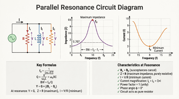
2. Parallel Resonance (Rejector Circuits)

When $I_L$ exactly equals $I_C$ in a parallel circuit, the net reactive current becomes zero. The total current drawn from the source is minimized and equals only the resistive current ($I_{total} = I_R$). At this specific frequency, the circuit’s impedance reaches its maximum value.

This phenomenon is called Parallel Resonance. Unlike series resonance (which maximizes current), parallel resonance minimizes it. Parallel resonant circuits are used as “rejector” circuits or band-stop filters to block specific unwanted frequencies (like radio interference) while allowing all other frequencies to pass.

3. Oscillators and RF Tuning

Parallel LC circuits (often called “tank circuits” because they store energy oscillating back and forth between the magnetic field of the inductor and the electric field of the capacitor) are the heart of radio frequency (RF) oscillators and tuning circuits. In a radio receiver, a parallel tank circuit is used to select the desired broadcast frequency while rejecting others.

4. Impedance Matching

In audio and telecommunications, parallel RLC networks are used to transform impedances, ensuring maximum power transfer between a source and a load by matching their complex impedance values.

Conclusion

The parallel RLC circuit completes our fundamental understanding of AC network analysis. By shifting our perspective from the constant current of series circuits to the constant voltage of parallel circuits, we unlock a new set of analytical tools, primarily the Current Triangle and the concept of Admittance.

Key takeaways from this guide include:

Reference Phasor: In a parallel circuit, voltage is constant across all branches and serves as the 0° reference phasor.
Branch Currents: Current is calculated individually for each branch ($I_R = V/R$, $I_L = V/X_L$, $I_C = V/X_C$).
Current Cancellation: The inductive and capacitive branch currents are 180° out of phase and subtract from one another. The total current is the vector sum of the resistive current and the net reactive current.
Impedance Rule: The total equivalent impedance of a parallel circuit is always less than the impedance of the smallest individual branch.
Phase Angle: The phase angle $\theta = \arctan(I_X / I_R)$ determines whether the total current leads (capacitive) or lags (inductive) the voltage.
Power Factor Correction: Parallel capacitors are used industrially to cancel out inductive lagging currents, improving system efficiency.

Mastering the analysis of the parallel RLC circuit provides you with the complete analytical framework required to tackle any linear AC network. Whether you are designing a power factor correction bank for a manufacturing plant, tuning an RF oscillator, or analyzing complex building electrical systems, the principles of parallel RLC analysis are the indispensable tools of the electrical engineer.