Power Factor Correction

Introduction to Power Factor Correction

In the modern industrial and commercial landscape, Power Factor Correction (PFC) has evolved from a niche engineering concern to a critical economic and operational necessity. As electrical systems become increasingly laden with inductive loads—motors, transformers, fluorescent lighting, and HVAC systems—the power factor of facilities often drops to inefficient levels, sometimes as low as 0.6 or 0.7.

This inefficiency comes at a steep price. Utilities charge industrial customers penalties for low power factor, equipment must be oversized to handle excess current, energy losses increase, and voltage regulation suffers. Power Factor Correction is the systematic approach to resolving these issues by adding reactive power compensation to the electrical system, typically using capacitor banks, to bring the power factor closer to unity (1.0).

This comprehensive guide will explore every aspect of power factor correction, from the fundamental principles to advanced automatic correction systems, capacitor bank sizing calculations, harmonic considerations, and economic analysis. Whether you’re an electrical engineer designing a new facility, a facility manager looking to reduce energy costs, or a student mastering AC power systems, this guide provides the complete toolkit for effective power factor correction.

What is Power Factor Correction?
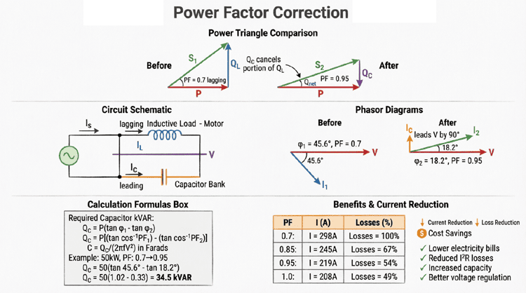
Power Factor Correction is the process of improving a facility’s power factor by adding reactive power compensation (typically capacitor banks) to counteract the inductive reactive power consumed by motors and other inductive loads. This reduces apparent power demand, lowers current, decreases energy losses, and avoids utility penalties.

Why Power Factor Correction is Essential

Before diving into the “how,” it’s crucial to understand the “why.” Low power factor creates multiple problems that directly impact operational costs and system reliability.

1. Utility Penalties and Increased Costs

Most industrial and commercial utility contracts include power factor clauses. If your facility’s average power factor drops below a specified threshold (typically 0.90 to 0.95 lagging), you face:

• kVA Demand Charges: Instead of billing based on kW (real power), the utility bills based on kVA (apparent power). Since kVA = kW / PF, a low PF dramatically increases your bill.
• Direct Penalties: Some utilities add a percentage surcharge for every 0.01 that PF drops below the threshold.
• Reactive Energy Charges: Some utilities separately bill for kVARh (reactive energy consumption).

Example Cost Impact:
A facility drawing 500 kW at PF = 0.70:

• Apparent Power: $S = 500 / 0.70 = 714 \text{ kVA}$
• If utility charges $15/kVA demand: $714 \times 15 = \$10,710/\text{month}$

Same facility corrected to PF = 0.95:

• Apparent Power: $S = 500 / 0.95 = 526 \text{ kVA}$
• Demand charge: $526 \times 15 = \$7,890/\text{month}$

Monthly Savings: \$2,820 | Annual Savings: \$33,840

2. Increased System Capacity

By improving power factor, you effectively free up capacity in your existing electrical infrastructure:

• Transformers: A 1000 kVA transformer operating at PF = 0.70 can only deliver 700 kW of real power. At PF = 0.95, it can deliver 950 kW—a 36% increase in usable capacity without upgrading equipment.
• Switchgear and Breakers: Lower current means existing protective devices can handle more real power load.
• Conductors: Reduced current decreases heating, potentially allowing existing cables to carry more load.

This “virtual capacity” often defers or eliminates the need for expensive infrastructure upgrades.

3. Reduced Energy Losses

Power losses in conductors, transformers, and switchgear are proportional to the square of the current ($I^2R$). By reducing current through power factor correction, you dramatically reduce these losses.

Loss Reduction Formula:
$\text{Loss Reduction} \% = 100 \times \left[1 – \left(\frac{PF_1}{PF_2}\right)^2\right]$

Improving PF from 0.70 to 0.95:
$\text{Loss Reduction} = 100 \times \left[1 – \left(\frac{0.70}{0.95}\right)^2\right] = 100 \times [1 – 0.54] = 46\%$

Nearly half the $I^2R$ losses are eliminated!

4. Improved Voltage Regulation

Low power factor causes higher voltage drops across distribution lines and transformers ($V_{drop} = I \times Z$). By reducing current, power factor correction:

• Maintains voltage levels closer to nominal
• Reduces voltage fluctuations
• Improves motor performance and lifespan
• Prevents nuisance tripping of sensitive equipment

Methods of Power Factor Correction

Several technologies exist for power factor correction, each with specific applications and advantages.

1. Shunt Capacitor Banks (Most Common)

Fixed Capacitor Banks:

• Permanently connected capacitors sized for base load
• Simple, low-cost, reliable
• Best for facilities with constant, predictable loads
• Risk of over-correction during light load periods

Automatic/Switched Capacitor Banks:

• Multiple capacitor steps controlled by a Power Factor Relay
• Automatically switches capacitors in/out based on real-time PF
• Maintains target PF (e.g., 0.95) under varying load conditions
• More expensive but highly effective for variable loads

Advantages:

• Low cost per kVAR
• Simple installation and maintenance
• Low losses (< 0.5 W/kVAR)
• Long service life (15-20 years)

Disadvantages:

• Can create resonance with system inductance
• Performance degrades with voltage and frequency variations
• Limited control granularity (stepped correction)

2. Synchronous Condensers

A synchronous motor running without mechanical load, over-excited to generate reactive power.

Advantages:

• Continuously variable reactive power control
• Can absorb or generate VARs (leading or lagging)
• Provides system inertia and stability
• Robust and durable

Disadvantages:

• High capital cost
• Requires regular maintenance
• Higher losses than capacitors
• Large physical footprint

Applications: Utility substations, large industrial facilities requiring dynamic VAR control.

3. Static VAR Compensators (SVC)

Power electronics-based systems using thyristor-controlled reactors (TCR) and thyristor-switched capacitors (TSC).

Advantages:

• Very fast response (< 1 cycle)
• Continuously variable control
• Can handle rapid load fluctuations
• No resonance issues

Disadvantages:

• High cost
• Generates harmonics (requires filters)
• Complex control systems
• Higher losses than capacitors

Applications: Arc furnaces, welding plants, facilities with rapidly fluctuating loads.

4. Active Power Factor Correction (APFC)

Used primarily at the equipment level (inside power supplies, VFDs, etc.). Uses boost converters and PWM control to shape input current into a sine wave in phase with voltage.

Advantages:

• Near-unity power factor (0.99+)
• Eliminates harmonic distortion
• Wide input voltage range
• Compact size

Disadvantages:

• Higher cost per unit
• Only practical for individual equipment
• Not suitable for facility-wide correction

Applications: Computer power supplies, LED drivers, variable frequency drives.

What is the most common method of power factor correction?
Shunt capacitor banks are the most common method due to their low cost, simplicity, and reliability. They can be fixed (for constant loads) or automatic/switched (for variable loads). Capacitors typically cost $15-$50 per kVAR and can last 15-20 years with minimal maintenance.

Capacitor Bank Sizing and Calculations

Properly sizing a capacitor bank is critical. Undersizing won’t achieve the target power factor, while oversizing can cause over-voltage, leading power factor, and resonance problems.

Step-by-Step Sizing Method

Step 1: Gather Load Data

• Real power demand ($P$) in kW
• Existing power factor ($PF_1$)
• Target power factor ($PF_2$)
• System voltage ($V$)
• System frequency ($f$)

Step 2: Calculate Phase Angles
$\theta_1 = \arccos(PF_1)$
$\theta_2 = \arccos(PF_2)$

Step 3: Calculate Required Capacitor kVAR
$Q_c = P \times (\tan(\theta_1) – \tan(\theta_2))$

Step 4: Verify Capacitor Current
$I_c = \frac{Q_c \times 1000}{\sqrt{3} \times V_{LL}}$ (for 3-phase)

Step 5: Check for Over-Correction
Ensure $Q_c < Q_{load}$ to avoid leading power factor at minimum load.

Practical Example: Industrial Facility

Problem: A manufacturing plant has the following characteristics:

• Average demand: 800 kW
• Existing power factor: 0.78 lagging
• Target power factor: 0.95 lagging
• System: 480V, 3-phase, 60 Hz
• Minimum load: 300 kW

Calculate the required capacitor bank size and verify it won’t over-correct at minimum load.

Solution:

Step 1: Calculate Phase Angles
$\theta_1 = \arccos(0.78) = 38.74^\circ$
$\theta_2 = \arccos(0.95) = 18.19^\circ$

Step 2: Find Tangents
$\tan(38.74^\circ) = 0.802$
$\tan(18.19^\circ) = 0.329$

Step 3: Calculate Required kVAR
$Q_c = 800 \times (0.802 – 0.329)$
$Q_c = 800 \times 0.473$
$Q_c = 378.4 \text{ kVAR}$

Step 4: Calculate Capacitor Current
$I_c = \frac{378.4 \times 1000}{\sqrt{3} \times 480}$
$I_c = \frac{378,400}{831.4}$
$I_c = 455 \text{ A}$

Step 5: Check Minimum Load Condition
At minimum load (300 kW), with existing PF = 0.78:
$Q_{min} = 300 \times \tan(38.74^\circ) = 300 \times 0.802 = 240.6 \text{ kVAR}$

If we install 378 kVAR capacitors:
$Q_{net} = 240.6 – 378 = -137.4 \text{ kVAR}$ (leading!)

Problem: The capacitor bank would over-correct at minimum load, creating a leading power factor.

Solution: Use an automatic capacitor bank with multiple steps:

• Total capacity: 378 kVAR
• Configuration: 6 steps of 63 kVAR each
• Controller switches steps based on real-time PF
• Prevents over-correction during light loads

Capacitor Bank Configuration

Delta vs. Wye Connection:

Delta Connection:

• Lower capacitor current for same kVAR
• Better for low voltage systems (< 600V)
• Continues operating if one capacitor fails (open delta)
• Capacitors rated for line-to-line voltage

Wye (Star) Connection:

• Better for high voltage systems (> 600V)
• Lower voltage stress on capacitors
• Easier to detect failures
• Neutral point available for grounding

Standard Practice:

• 480V systems: Delta connection
• 4160V and above: Wye connection

Automatic Power Factor Correction (APFC) Systems

For facilities with varying loads, Automatic Power Factor Correction (APFC) systems are essential. These systems use intelligent controllers to switch capacitor steps in and out, maintaining the target power factor under all load conditions.

Components of an APFC System

1. Power Factor Relay/Controller:

• Measures real-time voltage, current, and power factor
• Calculates required reactive power compensation
• Controls capacitor contactors based on setpoints
• Typically has 6-18 output steps

2. Capacitor Steps:

• Individual capacitor units (e.g., 25 kVAR, 50 kVAR)
• Each step controlled by a contactor
• Sized in binary progression (1:2:4:8…) or equal steps

3. Contactors:

• Capacitor-duty contactors (not standard motor contactors)
• Rated for high inrush currents
• Include pre-insertion resistors or reactors to limit switching transients

4. Current Transformer (CT):

• Provides current signal to controller
• Must be installed on the main incoming feeder
• Proper polarity is critical

5. Protection Devices:

• Overcurrent protection (fuses or breakers)
• Overvoltage protection
• Temperature monitoring
• Harmonic filters (if needed)

Control Strategies

1. Power Factor Control (Most Common):

• Maintains PF within a band (e.g., 0.95 to 0.98 lagging)
• Simple and effective for most applications

2. kVAR Control:

• Maintains reactive power demand below a setpoint
• Useful when utility charges for kVAR demand

3. Voltage Control:

• Switches capacitors to maintain voltage levels
• Often combined with PF control

4. Time-Based Control:

• Switches based on time-of-day schedules
• Useful for predictable load patterns

APFC System Design Example

Facility: Commercial office building

• Peak demand: 600 kW
• Minimum demand: 150 kW
• Existing PF: 0.75
• Target PF: 0.96
• Voltage: 480V, 3-phase

Step 1: Calculate Total kVAR Required
$\theta_1 = \arccos(0.75) = 41.41^\circ$
$\theta_2 = \arccos(0.96) = 16.26^\circ$
$Q_c = 600 \times (\tan(41.41^\circ) – \tan(16.26^\circ))$
$Q_c = 600 \times (0.882 – 0.292) = 600 \times 0.590$
$Q_c = 354 \text{ kVAR}$

Step 2: Select Step Configuration
Using 8-step binary configuration:

• Step 1: 25 kVAR
• Step 2: 25 kVAR
• Step 3: 50 kVAR
• Step 4: 50 kVAR
• Step 5: 50 kVAR
• Step 6: 50 kVAR
• Step 7: 50 kVAR
• Step 8: 54 kVAR
• Total: 354 kVAR

This configuration provides fine control at low loads and coarse control at high loads.

Step 3: Verify Minimum Load
At 150 kW with PF = 0.75:
$Q_{load} = 150 \times 0.882 = 132.3 \text{ kVAR}$

Controller will only switch in steps as needed, preventing over-correction.

Harmonic Considerations in PFC

One of the most critical and often overlooked aspects of power factor correction is harmonic resonance. Capacitors and system inductance can form a resonant circuit that amplifies harmonic currents, potentially causing catastrophic equipment failure.

The Resonance Problem

The resonant frequency of a capacitor bank and system inductance is:

$f_r = f_1 \times \sqrt{\frac{S_{sc}}{Q_c}}$

Where:

• $f_r$ = Resonant frequency (Hz)
• $f_1$ = Fundamental frequency (50 or 60 Hz)
• $S_{sc}$ = System short-circuit capacity (kVA)
• $Q_c$ = Capacitor bank size (kVAR)

If $f_r$ coincides with a dominant harmonic (typically 5th = 300 Hz, 7th = 420 Hz), severe resonance occurs.

Detuned Filters

To avoid resonance, detuned filters are used. These are capacitor banks with series reactors tuned below the lowest dominant harmonic (typically to 4.7th harmonic or 282 Hz for 60 Hz systems).

Reactor Sizing:
The reactor impedance is typically 5.67% to 7% of the capacitor impedance at fundamental frequency.

Advantages:

• Prevents resonance
• Protects capacitors from harmonic overload
• Provides some harmonic filtering
• Standard solution for facilities with VFDs or non-linear loads

Disadvantages:

• Higher cost (20-40% more than plain capacitors)
• Larger physical size
• Slightly higher losses

When to Use Detuned Filters

Use detuned filters when:

• Total harmonic distortion (THD) > 10%
• Significant non-linear loads present (VFDs, rectifiers, UPS)
• Multiple capacitor banks in the system
• History of capacitor failures or fuse blowing

Plain capacitors acceptable when:

• THD < 5%
• Predominantly linear loads (motors, heaters, lighting)
• Small capacitor banks (< 100 kVAR)

Economic Analysis and ROI

Power factor correction is one of the few electrical upgrades with a clear, rapid return on investment.

Cost Components

Capital Costs:

• Capacitor bank equipment: $15-$50 per kVAR
• Installation and labor: $5-$15 per kVAR
• Engineering and design: $2-$5 per kVAR
• Total installed cost: $25-$75 per kVAR

Annual Savings:

1. Reduced Demand Charges:
   $\text{Savings} = (kVA_{old} – kVA_{new}) \times \text{Rate} \times 12$
2. Reduced Energy Losses:
   $\text{Savings} = \text{Loss Reduction (kWh)} \times \text{Energy Rate}$
3. Avoided Penalties:
   Direct PF penalty charges eliminated
4. Deferred Infrastructure Upgrades:
   Harder to quantify but significant

ROI Calculation Example

Facility: 500 kW average demand

• Existing PF: 0.75
• Target PF: 0.95
• Utility demand charge: $15/kVA/month
• Energy cost: $0.10/kWh
• Hours of operation: 6,000 hours/year

Step 1: Calculate Required kVAR
$Q_c = 500 \times (\tan(\arccos(0.75)) – \tan(\arccos(0.95)))$
$Q_c = 500 \times (0.882 – 0.329) = 276.5 \text{ kVAR}$

Step 2: Calculate Capital Cost
Installed cost: $40/kVAR (mid-range)
Total cost: $276.5 \times 40 = \$11,060

Step 3: Calculate Annual Savings

Demand Charge Savings:
$kVA_{old} = 500 / 0.75 = 666.7 \text{ kVA}$
$kVA_{new} = 500 / 0.95 = 526.3 \text{ kVA}$
$\text{Reduction} = 140.4 \text{ kVA}$
$\text{Annual savings} = 140.4 \times 15 \times 12 = \$25,272$

Loss Reduction Savings:
Assume system losses = 3% of demand at PF = 0.75
Loss reduction ≈ 40% (from earlier formula)
$\text{Loss reduction} = 500 \text{ kW} \times 0.03 \times 0.40 = 6 \text{ kW}$
$\text{Annual energy savings} = 6 \times 6,000 \times 0.10 = \$3,600$

Total Annual Savings: \$25,272 + \$3,600 = \$28,872

Step 4: Calculate Payback Period
$\text{Payback} = \frac{\text{Capital Cost}}{\text{Annual Savings}} = \frac{11,060}{28,872} = 0.38 \text{ years}$

Payback: 4.6 months!

Even with conservative estimates, power factor correction typically pays for itself in 6-18 months.

Installation and Maintenance Best Practices

Installation Guidelines

Location:

• Install as close to the inductive load as possible
• For facility-wide correction: main service entrance or distribution panels
• Avoid areas with high ambient temperature (> 40°C)
• Ensure adequate ventilation

Protection:

• Overcurrent protection: 135-165% of capacitor rated current
• Overvoltage protection: capacitors rated 10-15% above system voltage
• Disconnecting means required for maintenance
• Grounding per NEC/local codes

Wiring:

• Use capacitor-duty contactors with pre-insertion resistors
• Size conductors for 135% of capacitor current
• Install current transformers for APFC controllers
• Verify CT polarity before energizing

Maintenance Requirements

Monthly:

• Visual inspection for bulging, leaks, or discoloration
• Check for unusual noise or vibration
• Verify APFC controller operation

Annually:

• Infrared thermography to detect hot connections
• Measure capacitance (should be within ±5% of nameplate)
• Check contactor operation and contact resistance
• Clean enclosures and ventilation openings
• Verify protective device settings

Every 5 Years:

• Comprehensive testing by qualified technician
• Consider replacement if capacitance has degraded > 10%
• Update settings if load profile has changed

Summary and Conclusion

Power Factor Correction is one of the most cost-effective electrical upgrades available to industrial and commercial facilities. By strategically adding capacitor banks to counteract inductive reactive power, facilities can achieve:

1. Immediate Cost Savings: Reduced demand charges and energy losses typically provide payback in 6-18 months
2. Increased Capacity: Existing infrastructure can handle 20-40% more real power load
3. Improved Reliability: Better voltage regulation and reduced heating extend equipment life
4. Regulatory Compliance: Meet utility power factor requirements and avoid penalties

Key takeaways from this guide include:

• Sizing: Use $Q_c = P \times (\tan(\theta_1) – \tan(\theta_2))$ to calculate required kVAR
• Technology: Fixed capacitors for constant loads; automatic systems for variable loads
• Harmonics: Always assess harmonic content; use detuned filters if THD > 10%
• Economics: ROI is typically excellent, with payback periods under 2 years
• Maintenance: Regular inspection and testing ensure long-term reliability

Whether you’re designing a new facility, retrofitting an existing installation, or simply looking to reduce energy costs, power factor correction should be a priority consideration. The combination of rapid payback, operational benefits, and improved system performance makes PFC one of the smartest investments in electrical efficiency.