Power in AC Circuits: Real, Reactive, and Apparent Power

Introduction to AC Power

Power in alternating current (AC) circuits is fundamentally different from power in direct current (DC) circuits. In DC systems, power calculation is straightforward: $P = V \times I$. However, in AC circuits, the continuous variation of voltage and current, combined with potential phase differences between them, creates a more complex power landscape.

AC power consists of three distinct but interrelated components:

• Real Power (P): The actual power that performs useful work, measured in watts (W)
• Reactive Power (Q): The power that oscillates between source and load, measured in volt-amperes reactive (VAR)
• Apparent Power (S): The total power supplied by the source, measured in volt-amperes (VA)

Understanding these power components is essential for:

• Designing efficient electrical systems
• Sizing equipment (generators, transformers, conductors)
• Calculating energy costs
• Improving power factor
• Ensuring system stability
• Meeting utility requirements

This comprehensive guide will explore all aspects of power in AC circuits, from instantaneous power to complex power calculations, complete with visual diagrams, practical examples, and real-world applications.

What are the three types of power in AC circuits?
Real power (P, in watts) performs useful work and is consumed by resistive loads. Reactive power (Q, in VAR) oscillates between source and load, creating magnetic/electric fields but doing no net work. Apparent power (S, in VA) is the total power supplied, combining both: S = √(P² + Q²).

Instantaneous Power in AC Circuits

Definition and Derivation

Instantaneous power is the power at any specific moment in time. It’s the product of instantaneous voltage and instantaneous current:

$p(t) = v(t) \times i(t)$

For a sinusoidal AC circuit with:

• $v(t) = V_m \sin(\omega t)$
• $i(t) = I_m \sin(\omega t – \theta)$

Where θ is the phase angle between voltage and current.

The instantaneous power becomes:

$p(t) = V_m I_m \sin(\omega t) \sin(\omega t – \theta)$

Using trigonometric identities, this expands to:

$p(t) = \frac{V_m I_m}{2} [\cos(\theta) – \cos(2\omega t – \theta)]$

Or in terms of RMS values ($V_{RMS} = V_m/\sqrt{2}$, $I_{RMS} = I_m/\sqrt{2}$):

$p(t) = V_{RMS} I_{RMS} [\cos(\theta) – \cos(2\omega t – \theta)]$

Characteristics of Instantaneous Power

The instantaneous power waveform has two components:

1. Constant (Average) Component:

• $V_{RMS} I_{RMS} \cos(\theta)$
• Represents the real power (P)
• Always positive (for passive loads)
• Does useful work

2. Oscillating Component:

• $-V_{RMS} I_{RMS} \cos(2\omega t – \theta)$
• Oscillates at twice the supply frequency
• Represents energy sloshing back and forth
• Average value = 0
• Associated with reactive power

Visualizing Instantaneous Power

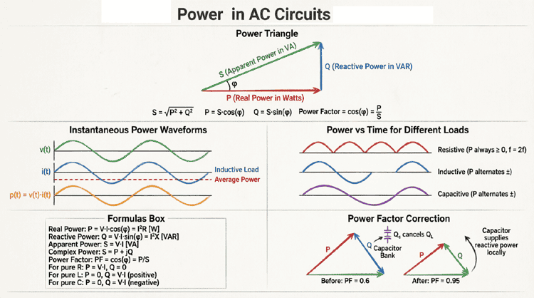
The instantaneous power:

• Is always positive when PF = 1 (purely resistive)
• Goes negative when PF < 1 (reactive components present)
• Has an average value equal to real power
• Oscillates at twice the line frequency (120 Hz for 60 Hz system)

Why does instantaneous power oscillate at twice the supply frequency?
Instantaneous power oscillates at 2× the supply frequency because it’s the product of two sine waves (voltage and current). When you multiply sin(ωt) × sin(ωt-θ), trigonometric identities show the result contains a cos(2ωt) term, creating oscillation at double the original frequency.

Real Power (Active Power)

Definition and Physical Meaning

Real power (also called active power or true power) is the component of AC power that performs actual work. It represents the average rate at which energy is transferred from the source to the load and converted into useful forms such as:

• Mechanical energy (motors)
• Heat (heaters, resistors)
• Light (lamps)
• Chemical energy (battery charging)

Real power is consumed by the load and is not returned to the source.

Calculation Formulas

General Formula:
$P = V_{RMS} \times I_{RMS} \times \cos(\theta)$

Where:

• P = Real power in watts (W)
• V_RMS = RMS voltage in volts (V)
• I_RMS = RMS current in amperes (A)
• cos(θ) = Power factor (PF)
• θ = Phase angle between voltage and current

Alternative Forms:

For resistive loads or when impedance is known:

$P = I_{RMS}^2 \times R$

$P = \frac{V_{RMS}^2}{R}$

Where R is the resistive component of the load.

From Apparent Power:
$P = S \times \cos(\theta)$

Where S is apparent power in VA.

Characteristics of Real Power

1. Always Positive: For passive loads, real power is always positive (energy flows from source to load)
2. Frequency Independent: Real power doesn’t oscillate; it’s the average value
3. Measurable: Can be measured with wattmeters
4. Billable: Utilities charge customers for real energy consumption (kWh)
5. Useful Work: Only real power performs actual work

Examples by Load Type

Purely Resistive Load (θ = 0°):

• $\cos(0°) = 1$
• $P = V_{RMS} \times I_{RMS}$
• All power is real power
• Example: Incandescent lamps, heaters

Purely Reactive Load (θ = 90°):

• $\cos(90°) = 0$
• $P = 0$
• No real power consumed
• Example: Ideal inductors, ideal capacitors

Mixed R-L or R-C Load (0° < θ < 90°):

• $0 < \cos(\theta) < 1$
• $P = V_{RMS} \times I_{RMS} \times \cos(\theta)$
• Partial real power
• Example: Motors, transformers, fluorescent lights

Reactive Power

Definition and Physical Meaning

Reactive power represents the energy that oscillates back and forth between the source and reactive components (inductors and capacitors) in the circuit. Unlike real power, reactive power:

• Is not consumed by the load
• Is stored temporarily in magnetic or electric fields
• Is returned to the source each cycle
• Performs no net work over a complete cycle

Despite not doing useful work, reactive power is essential for:

• Creating magnetic fields in motors and transformers
• Establishing electric fields in capacitors
• Maintaining voltage levels in power systems
• Enabling the operation of inductive loads

Calculation Formulas

General Formula:
$Q = V_{RMS} \times I_{RMS} \times \sin(\theta)$

Where:

• Q = Reactive power in volt-amperes reactive (VAR)
• V_RMS = RMS voltage in volts (V)
• I_RMS = RMS current in amperes (A)
• sin(θ) = Reactive factor
• θ = Phase angle between voltage and current

Alternative Forms:

For reactive loads:

$Q = I_{RMS}^2 \times X$

$Q = \frac{V_{RMS}^2}{X}$

Where X is the reactance (XL or XC).

From Apparent Power:
$Q = S \times \sin(\theta)$

Sign Convention

Inductive Loads (Current Lags Voltage):

• θ > 0
• $\sin(\theta) > 0$
• Q > 0 (positive reactive power)
• Inductors consume reactive power
• Also called “lagging” reactive power

Capacitive Loads (Current Leads Voltage):

• θ < 0
• $\sin(\theta) < 0$
• Q < 0 (negative reactive power)
• Capacitors supply reactive power
• Also called “leading” reactive power

Physical Interpretation

Inductor:

• Stores energy in magnetic field during one quarter-cycle
• Returns energy to source during next quarter-cycle
• Net energy transfer = 0
• But reactive power flow is necessary for magnetic field

Capacitor:

• Stores energy in electric field during one quarter-cycle
• Returns energy to source during next quarter-cycle
• Net energy transfer = 0
• But reactive power flow is necessary for electric field

What is the difference between real and reactive power?
Real power (P, in watts) performs actual work and is consumed by the load. Reactive power (Q, in VAR) oscillates between source and load, storing energy in magnetic/electric fields but doing no net work. Real power is billable; reactive power supports equipment operation but doesn’t directly perform work.

Apparent Power

Definition and Significance

Apparent power is the product of RMS voltage and RMS current, representing the total power that must be supplied by the source. It’s called “apparent” because it appears to be the total power, but it’s actually a combination of real and reactive power.

$S = V_{RMS} \times I_{RMS}$

Where:

• S = Apparent power in volt-amperes (VA)
• V_RMS = RMS voltage in volts (V)
• I_RMS = RMS current in amperes (A)

Why Apparent Power Matters

Apparent power is crucial for:

1. Equipment Sizing:

• Generators must supply both real and reactive power
• Transformers must handle total current (not just real power current)
• Conductors must be sized for total RMS current
• Circuit breakers must interrupt total current

2. System Capacity:

• Utility infrastructure is rated in kVA or MVA
• Determines maximum load a system can handle
• Independent of power factor

3. Voltage Regulation:

• Reactive power affects voltage drops
• Impacts system stability

Relationship to Real and Reactive Power

Apparent power is the vector sum (not arithmetic sum) of real and reactive power:

$S = \sqrt{P^2 + Q^2}$

This relationship forms the Power Triangle.

Conversely:

• $P = S \times \cos(\theta)$
• $Q = S \times \sin(\theta)$
• $S = P + jQ$ (complex form)

Units and Scaling

Common Units:

• VA (volt-amperes) – small equipment
• kVA (kilovolt-amperes) = 1,000 VA – transformers, generators
• MVA (megavolt-amperes) = 1,000,000 VA – power plants, substations

Example:
A 100 kVA transformer can supply:

• 100 kW at PF = 1.0
• 80 kW at PF = 0.8
• 60 kW at PF = 0.6

The transformer rating (kVA) stays constant, but usable real power (kW) depends on power factor.

The Power Triangle

Geometric Representation

The Power Triangle is a right triangle that visually represents the relationship between real power (P), reactive power (Q), and apparent power (S).

Triangle Relationships

Pythagorean Theorem:
$S^2 = P^2 + Q^2$

Power Factor:
$\cos(\theta) = \frac{P}{S}$

Reactive Factor:
$\sin(\theta) = \frac{Q}{S}$

Tangent Relationship:
$\tan(\theta) = \frac{Q}{P}$

Triangle Variations

Inductive Load (Lagging PF):

• Q is positive (points up)
• Current lags voltage
• Triangle in first quadrant

Capacitive Load (Leading PF):

• Q is negative (points down)
• Current leads voltage
• Triangle in fourth quadrant

Purely Resistive Load:

• Q = 0
• Triangle collapses to horizontal line
• S = P
• PF = 1.0

Purely Reactive Load:

• P = 0
• Triangle collapses to vertical line
• S = |Q|
• PF = 0

Power Factor

Definition and Importance

Power factor (PF) is the ratio of real power to apparent power:

$PF = \frac{P}{S} = \cos(\theta)$

Where θ is the phase angle between voltage and current.

Power factor indicates how effectively electrical power is being used:

• PF = 1.0 (unity): All power is real power (ideal)
• PF = 0: All power is reactive power (worst case)
• 0 < PF < 1: Mixture of real and reactive power

Types of Power Factor

Lagging Power Factor:

• Caused by inductive loads (motors, transformers)
• Current lags voltage
• Q > 0
• Most common in industrial facilities

Leading Power Factor:

• Caused by capacitive loads (capacitor banks, underground cables)
• Current leads voltage
• Q < 0
• Less common, sometimes intentional for correction

Unity Power Factor:

• Purely resistive load
• Current in phase with voltage
• Q = 0
• Ideal but rarely achieved in practice

Impact of Low Power Factor

Problems:

1. Increased Current:

• For same real power, lower PF requires higher current
• $I = \frac{P}{V \times PF}$
• Example: 10 kW at 240V
  • PF = 1.0 → I = 41.7A
  • PF = 0.7 → I = 59.5A (43% increase!)

2. Higher Losses:

• Power losses = I²R
• 43% more current = 105% more losses!

3. Larger Equipment:

• Conductors, transformers, breakers must be oversized
• Increased capital costs

4. Utility Penalties:

• Many utilities charge for PF < 0.9 or 0.95
• Increases electricity costs

5. Reduced System Capacity:

• Existing infrastructure handles less real power
• Wasted capacity

Power Factor Correction

Method: Add capacitors in parallel with inductive loads

Effect:

• Capacitors supply reactive power locally
• Reduce reactive power drawn from source
• Improve power factor
• Reduce current and losses

Calculation:
Required capacitor kVAR = $P \times (\tan(\theta_1) – \tan(\theta_2))$

Where:

• θ₁ = initial phase angle
• θ₂ = target phase angle

Complex Power

Mathematical Representation

Complex power combines real and reactive power into a single complex number:

$\mathbf{S} = P + jQ$

Where:

• S = Complex power in VA
• P = Real power in W (real part)
• Q = Reactive power in VAR (imaginary part)
• j = Imaginary unit (√-1)

Polar Form

Complex power can also be expressed in polar form:

$\mathbf{S} = S \angle \theta = S (\cos(\theta) + j\sin(\theta))$

Where:

• S = Magnitude (apparent power)
• θ = Phase angle

Calculation from Phasors

If voltage and current are expressed as phasors:

• $\mathbf{V} = V \angle \theta_v$
• $\mathbf{I} = I \angle \theta_i$

Then complex power is:

$\mathbf{S} = \mathbf{V} \times \mathbf{I}^*$

Where I* is the complex conjugate of current.

This gives:
$\mathbf{S} = V I \angle (\theta_v – \theta_i) = V I \angle \theta$

Which separates into:
$\mathbf{S} = VI\cos(\theta) + jVI\sin(\theta) = P + jQ$

Advantages of Complex Power

1. Simplified Calculations:

• Combine P and Q in one quantity
• Easy to add powers from multiple loads
• $\mathbf{S}_{total} = \mathbf{S}_1 + \mathbf{S}_2 + … + \mathbf{S}_n$

2. Circuit Analysis:

• Use complex algebra
• Apply circuit theorems
• Simplify power flow studies

3. Complete Information:

• Magnitude gives apparent power
• Real part gives real power
• Imaginary part gives reactive power
• Angle gives power factor

Single-Phase vs. Three-Phase Power

Single-Phase Power

Real Power:
$P_{1\phi} = V_{RMS} \times I_{RMS} \times \cos(\theta)$

Reactive Power:
$Q_{1\phi} = V_{RMS} \times I_{RMS} \times \sin(\theta)$

Apparent Power:
$S_{1\phi} = V_{RMS} \times I_{RMS}$

Used in:

• Residential applications
• Small commercial loads
• Light industrial equipment

Three-Phase Power (Balanced System)

For balanced three-phase systems:

Real Power:
$P_{3\phi} = \sqrt{3} \times V_L \times I_L \times \cos(\theta)$

Or using phase quantities:
$P_{3\phi} = 3 \times V_{phase} \times I_{phase} \times \cos(\theta)$

Reactive Power:
$Q_{3\phi} = \sqrt{3} \times V_L \times I_L \times \sin(\theta)$

Apparent Power:
$S_{3\phi} = \sqrt{3} \times V_L \times I_L$

Where:

• V_L = Line-to-line voltage
• I_L = Line current
• θ = Phase angle (same for all phases in balanced system)

Advantages of Three-Phase Power

1. More Power for Same Current:

• 3-phase delivers √3 (1.732) times more power than single-phase
• For same voltage and current

2. Constant Power:

• Instantaneous power is constant (doesn’t pulsate)
• Smoother motor operation
• Less vibration

3. Efficient:

• Less conductor material for same power
• Better utilization of equipment

4. Self-Starting Motors:

• Three-phase motors are self-starting
• No need for starting capacitors or mechanisms

Practical Examples and Calculations

Example 1: Calculating Power Components

Problem: A single-phase motor draws 15A from a 240V, 60Hz supply. The current lags the voltage by 36.87°. Calculate real power, reactive power, apparent power, and power factor.

Solution:

Given:

• $V_{RMS} = 240\text{V}$
• $I_{RMS} = 15\text{A}$
• $\theta = 36.87°$ (lagging)

Calculate Apparent Power:
$S = V_{RMS} \times I_{RMS}$
$S = 240 \times 15$
$S = 3,600 \text{ VA} = 3.6 \text{ kVA}$

Calculate Real Power:
$P = V_{RMS} \times I_{RMS} \times \cos(\theta)$
$P = 240 \times 15 \times \cos(36.87°)$
$P = 3,600 \times 0.8$
$P = 2,880 \text{ W} = 2.88 \text{ kW}$

Calculate Reactive Power:
$Q = V_{RMS} \times I_{RMS} \times \sin(\theta)$
$Q = 240 \times 15 \times \sin(36.87°)$
$Q = 3,600 \times 0.6$
$Q = 2,160 \text{ VAR} = 2.16 \text{ kVAR}$ (inductive)

Calculate Power Factor:
$PF = \cos(\theta) = \cos(36.87°)$
$PF = 0.8$ (lagging)

Verify Power Triangle:
$S = \sqrt{P^2 + Q^2}$
$S = \sqrt{2,880^2 + 2,160^2}$
$S = \sqrt{8,294,400 + 4,665,600}$
$S = \sqrt{12,960,000}$
$S = 3,600 \text{ VA}$ ✓

Example 2: Three-Phase Power Calculation

Problem: A balanced three-phase load is connected to a 480V line-to-line supply. Each phase draws 50A at a power factor of 0.85 lagging. Calculate total real power, reactive power, and apparent power.

Solution:

Given:

• $V_L = 480\text{V}$
• $I_L = 50\text{A}$
• $PF = 0.85$ (lagging)

Find Phase Angle:
$\theta = \arccos(0.85)$
$\theta = 31.79°$

Calculate Real Power:
$P_{3\phi} = \sqrt{3} \times V_L \times I_L \times \cos(\theta)$
$P_{3\phi} = 1.732 \times 480 \times 50 \times 0.85$
$P_{3\phi} = 35,330 \text{ W} = 35.33 \text{ kW}$

Calculate Reactive Power:
$Q_{3\phi} = \sqrt{3} \times V_L \times I_L \times \sin(\theta)$
$Q_{3\phi} = 1.732 \times 480 \times 50 \times \sin(31.79°)$
$Q_{3\phi} = 1.732 \times 480 \times 50 \times 0.527$
$Q_{3\phi} = 21,890 \text{ VAR} = 21.89 \text{ kVAR}$

Calculate Apparent Power:
$S_{3\phi} = \sqrt{3} \times V_L \times I_L$
$S_{3\phi} = 1.732 \times 480 \times 50$
$S_{3\phi} = 41,570 \text{ VA} = 41.57 \text{ kVA}$

Verify:
$S = \sqrt{P^2 + Q^2}$
$S = \sqrt{35,330^2 + 21,890^2}$
$S = \sqrt{1,248,208,900 + 479,172,100}$
$S = \sqrt{1,727,381,000}$
$S = 41,560 \text{ VA}$ ✓ (minor rounding difference)

Example 3: Power Factor Correction

Problem: An industrial facility has a load of 500 kW at 0.75 lagging power factor. Calculate the capacitor kVAR required to improve the power factor to 0.95 lagging.

Solution:

Given:

• $P = 500 \text{ kW}$
• $PF_1 = 0.75$ (initial)
• $PF_2 = 0.95$ (target)

Step 1: Initial Conditions
$\theta_1 = \arccos(0.75) = 41.41°$
$Q_1 = P \times \tan(\theta_1)$
$Q_1 = 500 \times \tan(41.41°)$
$Q_1 = 500 \times 0.882$
$Q_1 = 441 \text{ kVAR}$ (inductive)

Initial apparent power:
$S_1 = P / PF_1 = 500 / 0.75 = 666.7 \text{ kVA}$

Step 2: Target Conditions
$\theta_2 = \arccos(0.95) = 18.19°$
$Q_2 = P \times \tan(\theta_2)$
$Q_2 = 500 \times \tan(18.19°)$
$Q_2 = 500 \times 0.329$
$Q_2 = 164.5 \text{ kVAR}$ (inductive)

Step 3: Required Capacitor Bank
The capacitor must supply the difference:
$Q_{capacitor} = Q_1 – Q_2$
$Q_{capacitor} = 441 – 164.5$
$Q_{capacitor} = 276.5 \text{ kVAR}$ (capacitive)

Step 4: Verify New Apparent Power
$S_2 = \sqrt{P^2 + Q_2^2}$
$S_2 = \sqrt{500^2 + 164.5^2}$
$S_2 = \sqrt{250,000 + 27,060}$
$S_2 = \sqrt{277,060}$
$S_2 = 526.4 \text{ kVA}$

Result: By adding a 276.5 kVAR capacitor bank:

• Apparent power reduced from 666.7 kVA to 526.4 kVA
• Current reduced by 21%
• Power factor improved from 0.75 to 0.95

Summary and Conclusion

Power in AC circuits is a multifaceted concept that extends far beyond the simple P = VI relationship of DC circuits. Understanding the interplay between real power, reactive power, and apparent power is essential for designing efficient electrical systems, optimizing energy usage, and ensuring reliable operation.

Key takeaways from this guide include:

1. Three Types of Power:

• Real power (P, watts): Performs useful work
• Reactive power (Q, VAR): Supports magnetic/electric fields
• Apparent power (S, VA): Total power supplied

2. Power Triangle:

• $S^2 = P^2 + Q^2$
• Visual representation of power relationships
• Foundation for power factor calculations

3. Power Factor:

• $PF = \cos(\theta) = P/S$
• Critical for system efficiency
• Low PF increases costs and reduces capacity

4. Instantaneous vs. Average Power:

• Instantaneous power oscillates at 2× line frequency
• Average power equals real power
• Reactive power causes oscillation

5. Complex Power:

• $\mathbf{S} = P + jQ$
• Simplifies calculations and analysis
• Combines all power components

6. Three-Phase Power:

• $P_{3\phi} = \sqrt{3} V_L I_L \cos(\theta)$
• More efficient than single-phase
• Standard for industrial applications

7. Power Factor Correction:

• Capacitors reduce reactive power demand
• Improve efficiency and reduce costs
• Essential for industrial facilities

Mastering AC power concepts enables you to design efficient electrical systems, troubleshoot power quality issues, optimize energy consumption, and make informed decisions about equipment sizing and power factor correction. Whether you’re working with residential wiring, industrial motor controls, or utility-scale power systems, the principles outlined in this guide form the foundation of effective electrical engineering practice.