Series Resonance Circuit
Series Resonance Circuit: Resonant Frequency and Q Factor
Introduction to Series Resonance
Resonance is one of the most fascinating and powerful phenomena in electrical engineering. It occurs when a system oscillates with maximum amplitude at a specific frequency, known as the resonant frequency. In AC circuits, resonance happens when the inductive and capacitive reactances become equal in magnitude but opposite in phase, effectively canceling each other out.
A Series Resonance Circuit (also called a Series RLC Circuit at resonance) exhibits unique characteristics that make it indispensable in countless applications. At resonance, the circuit impedance drops to its minimum value (equal to just the resistance), allowing maximum current to flow. This property is exploited in radio tuners to select specific frequencies, in filters to pass or block certain signals, and in power systems to avoid dangerous overcurrent conditions.
Understanding series resonance is crucial for designing efficient filters, tuning circuits, and avoiding potentially destructive resonance conditions in power systems. This comprehensive guide will explore the physics, mathematics, and practical applications of series resonance circuits, complete with visual diagrams and step-by-step calculations.
What is Series Resonance?
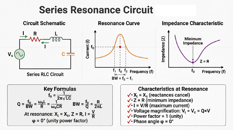
Series resonance occurs in an RLC circuit when the inductive reactance (X_L) equals the capacitive reactance (X_C). At this resonant frequency, the two reactances cancel each other out, leaving only the resistance to oppose current flow. This results in minimum impedance, maximum current, and a power factor of unity (1.0).
The Physics of Series Resonance
Understanding Reactance Cancellation
In a series RLC circuit, we have three components connected in a single loop: a resistor (R), an inductor (L), and a capacitor (C). Each component affects the circuit differently:
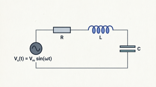
and capacitor (C) connected in series with AC voltage source Vs(t) = Vm sin(ωt)
- Resistor (R): Opposes current flow uniformly at all frequencies, with voltage and current in phase.
- Inductor (L): Creates inductive reactance ($X_L = 2\pi fL$) that increases with frequency. Voltage leads current by 90°.
- Capacitor (C): Creates capacitive reactance ($X_C = 1/(2\pi fC)$) that decreases with frequency. Current leads voltage by 90°.
The key to resonance lies in the frequency dependence of $X_L$ and $X_C$. As frequency increases:
- $X_L$ increases linearly
- $X_C$ decreases inversely
There must be one specific frequency where these two opposing reactances are exactly equal:
$X_L = X_C$
At this frequency, the inductive and capacitive voltages are equal in magnitude but 180° out of phase, meaning they completely cancel each other out in the phasor sum.
The Resonant Frequency Formula
Setting $X_L = X_C$ and solving for frequency gives us the resonant frequency formula:
$2\pi f_r L = \frac{1}{2\pi f_r C}$
Solving for $f_r$:
$f_r = \frac{1}{2\pi\sqrt{LC}}$
Where:
- $f_r$ = Resonant frequency in Hertz (Hz)
- $L$ = Inductance in Henrys (H)
- $C$ = Capacitance in Farads (F)
- $\pi$ = Pi (approximately 3.14159)
Alternatively, using angular frequency ($\omega_r = 2\pi f_r$):
$\omega_r = \frac{1}{\sqrt{LC}}$
This elegant formula shows that the resonant frequency depends only on the inductance and capacitance values, not on the resistance. The resistance affects the “sharpness” of resonance (Q factor) but not the resonant frequency itself.
How do you calculate resonant frequency?
The resonant frequency is calculated using the formula: f_r = 1/(2π√LC), where L is inductance in Henrys and C is capacitance in Farads. At this frequency, inductive reactance equals capacitive reactance, and the circuit impedance is minimum.
Characteristics of Series Resonance
1. Minimum Impedance
At resonance, since $X_L = X_C$, the net reactance becomes zero:
$X = X_L – X_C = 0$
Therefore, the total impedance is:
$Z = \sqrt{R^2 + (X_L – X_C)^2} = \sqrt{R^2 + 0^2} = R$
This is the minimum possible impedance for the circuit. The circuit behaves as a purely resistive load, even though it contains inductors and capacitors.
2. Maximum Current
Since impedance is minimum at resonance, the current drawn from the source reaches its maximum value:
$I_{max} = \frac{V}{R}$
This is significantly higher than the current at frequencies above or below resonance. This property makes series resonance circuits ideal for applications requiring high current at a specific frequency.
3. Unity Power Factor
At resonance, the circuit is purely resistive because the reactive components cancel out. This means:
- Voltage and current are in phase (0° phase difference)
- Power factor = $\cos(0°) = 1.0$ (unity)
- All power drawn from the source is real power (no reactive power)
4. Voltage Magnification
One of the most remarkable features of series resonance is voltage magnification. Even though the source voltage might be modest, the voltages across the inductor and capacitor can be many times larger than the source voltage!
At resonance:
- $V_L = I_{max} \times X_L$
- $V_C = I_{max} \times X_C$
Since $I_{max} = V/R$ and $X_L = X_C$ at resonance:
$V_L = V_C = \frac{V}{R} \times X_L = V \times \frac{X_L}{R}$
The ratio $X_L/R$ (or $X_C/R$) is called the Quality Factor (Q), which we’ll explore in detail later. If Q = 50, then the voltage across the inductor or capacitor will be 50 times the source voltage!
This voltage magnification is crucial in applications like radio receivers, where weak signals need to be amplified, but it can also be dangerous in power systems if not properly controlled.
Visualizing Series Resonance
Impedance vs. Frequency Curve
The impedance of a series RLC circuit varies dramatically with frequency. At resonance, impedance is minimum (equal to R). As frequency moves away from resonance (either higher or lower), the impedance increases.
The impedance curve shows:
- Below resonance ($f < f_r$): Capacitive reactance dominates ($X_C > X_L$), impedance is high and capacitive
- At resonance ($f = f_r$): Reactances cancel, impedance is minimum (= R)
- Above resonance ($f > f_r$): Inductive reactance dominates ($X_L > X_C$), impedance is high and inductive
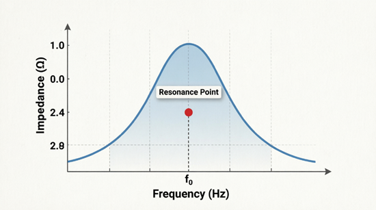
resonant frequency f₀. The circuit exhibits minimum impedance (equal to R) at
resonance and higher impedance at frequencies above or below resonance.
Current vs. Frequency Curve
The current curve is the inverse of the impedance curve. Since $I = V/Z$:
- At resonance: Current is maximum ($I_{max} = V/R$)
- Away from resonance: Current decreases as impedance increases
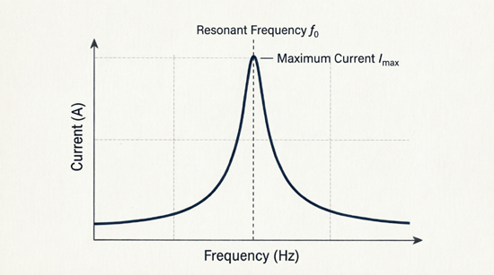
resonant frequency f₀. The sharp peak indicates high selectivity, with current
dropping to 70.7% of maximum at the half-power frequencies f₁ and f₂.
The sharpness of the current peak depends on the circuit’s Q factor. Higher Q means a sharper, narrower peak.
Phasor Diagram at Resonance
At resonance, the phasor diagram reveals the beautiful symmetry of the circuit:
- $V_R$ is horizontal (in phase with current)
- $V_L$ points straight up (leading current by 90°)
- $V_C$ points straight down (lagging current by 90°)
- $V_L$ and $V_C$ are equal in magnitude and opposite in direction
- The source voltage $V_S$ equals $V_R$ (since $V_L$ and $V_C$ cancel)
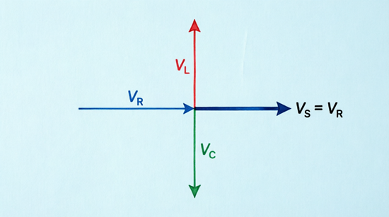
in phase with current, VL (inductor voltage) leading by 90°, and VC (capacitor voltage)
lagging by 90°. At resonance, VL and VC are equal and opposite, canceling each other,
making VS = VR.
Quality Factor (Q Factor) and Bandwidth
The Quality Factor (Q)
The Quality Factor or Q factor is a dimensionless parameter that describes how “sharp” or “selective” the resonance is. It is defined as the ratio of the resonant frequency to the bandwidth, or equivalently, as the ratio of reactance to resistance at resonance:
$Q = \frac{X_L}{R} = \frac{X_C}{R} = \frac{\omega_r L}{R} = \frac{1}{\omega_r RC}$
Where:
- $Q$ = Quality factor (dimensionless)
- $X_L$ = Inductive reactance at resonance
- $X_C$ = Capacitive reactance at resonance
- $R$ = Resistance
- $\omega_r$ = Angular resonant frequency
Physical Meaning of Q Factor
The Q factor has several important interpretations:
- Voltage Magnification: Q represents how many times the voltage across L or C is magnified compared to the source voltage. If Q = 100, then $V_L = V_C = 100 \times V_{source}$.
- Selectivity: Higher Q means the circuit is more selective—it responds strongly only to frequencies very close to $f_r$ and rejects frequencies even slightly away from resonance.
- Energy Storage: Q represents the ratio of energy stored in the reactive components to the energy dissipated in the resistor per cycle. High Q means low energy loss relative to energy stored.
Bandwidth (BW)
Bandwidth is the range of frequencies over which the circuit response (current) is at least 70.7% (or $1/\sqrt{2}$) of the maximum value at resonance. These points are called the half-power points or -3dB points.
The bandwidth is inversely proportional to the Q factor:
$BW = f_2 – f_1 = \frac{f_r}{Q}$
Where:
- $BW$ = Bandwidth in Hertz
- $f_2$ = Upper cutoff frequency (higher -3dB point)
- $f_1$ = Lower cutoff frequency (lower -3dB point)
- $f_r$ = Resonant frequency
- $Q$ = Quality factor
Cutoff Frequencies
The half-power frequencies can be calculated as:
$f_1 = f_r – \frac{BW}{2}$ (Lower cutoff)
$f_2 = f_r + \frac{BW}{2}$ (Upper cutoff)
At these frequencies:
- Current = $0.707 \times I_{max}$
- Impedance = $\sqrt{2} \times R$
- Power = $0.5 \times P_{max}$
Relationship Between Q, Bandwidth, and Selectivity
- High Q (> 10): Narrow bandwidth, sharp resonance peak, highly selective circuit. Used in radio tuners and filters requiring precise frequency selection.
- Low Q (< 10): Wide bandwidth, broad resonance peak, less selective circuit. Used in applications requiring wider frequency response.
What is the Q factor in a series resonance circuit?
The Q factor (Quality factor) is the ratio of reactance to resistance at resonance: Q = X_L/R = X_C/R. It indicates how selective the circuit is and how much voltage magnification occurs. Higher Q means sharper resonance, narrower bandwidth, and greater voltage magnification across L and C.
Step-by-Step Practical Example
Let’s work through a complete series resonance circuit analysis.
Problem Statement:
A series RLC circuit has the following components:
- Resistor: $R = 10 \Omega$
- Inductor: $L = 100 \text{ mH} = 0.1 \text{ H}$
- Capacitor: $C = 10 \text{ μF} = 10 \times 10^{-6} \text{ F}$
- Supply voltage: $V = 100\text{V (RMS)}$
Calculate:
- Resonant frequency ($f_r$)
- Inductive and capacitive reactance at resonance
- Circuit impedance at resonance
- Maximum current at resonance
- Quality factor (Q)
- Bandwidth (BW)
- Lower and upper cutoff frequencies ($f_1$ and $f_2$)
- Voltages across each component at resonance
Solution:
Step 1: Calculate Resonant Frequency
$f_r = \frac{1}{2\pi\sqrt{LC}}$
$f_r = \frac{1}{2\pi\sqrt{0.1 \times 10 \times 10^{-6}}}$
$f_r = \frac{1}{2\pi\sqrt{1 \times 10^{-6}}}$
$f_r = \frac{1}{2\pi \times 0.001}$
$f_r = \frac{1}{0.006283}$
$f_r \approx 159.15 \text{ Hz}$
Step 2: Calculate Reactances at Resonance
At resonance, $X_L = X_C$:
$X_L = 2\pi f_r L = 2\pi \times 159.15 \times 0.1$
$X_L = X_C \approx 100 \Omega$
Step 3: Calculate Impedance at Resonance
At resonance, $Z = R$:
$Z = 10 \Omega$
Step 4: Calculate Maximum Current
$I_{max} = \frac{V}{R} = \frac{100\text{V}}{10\Omega}$
$I_{max} = 10 \text{ A}$
Step 5: Calculate Quality Factor
$Q = \frac{X_L}{R} = \frac{100\Omega}{10\Omega}$
$Q = 10$
Step 6: Calculate Bandwidth
$BW = \frac{f_r}{Q} = \frac{159.15}{10}$
$BW = 15.915 \text{ Hz}$
Step 7: Calculate Cutoff Frequencies
$f_1 = f_r – \frac{BW}{2} = 159.15 – \frac{15.915}{2}$
$f_1 \approx 151.19 \text{ Hz}$
$f_2 = f_r + \frac{BW}{2} = 159.15 + \frac{15.915}{2}$
$f_2 \approx 167.11 \text{ Hz}$
Step 8: Calculate Component Voltages at Resonance
- Resistor Voltage: $V_R = I_{max} \times R = 10 \times 10 = \mathbf{100\text{V}}$
- Inductor Voltage: $V_L = I_{max} \times X_L = 10 \times 100 = \mathbf{1000\text{V}}$
- Capacitor Voltage: $V_C = I_{max} \times X_C = 10 \times 100 = \mathbf{1000\text{V}}$
Notice the voltage magnification! The source voltage is only 100V, but the voltages across the inductor and capacitor are each 1000V—ten times higher! This is the Q factor in action ($Q = 10$).
Practical Applications of Series Resonance
1. Radio and TV Tuners
Series resonance circuits are the heart of radio and television receivers. By using a variable capacitor (or variable inductor), the resonant frequency can be adjusted to match the frequency of the desired radio station. At resonance, the circuit allows maximum current to flow for that specific frequency while rejecting all others, effectively “tuning in” to the station.
2. Band-Pass Filters
Series resonance circuits are used as band-pass filters in audio equipment, communication systems, and signal processing. They allow frequencies within the bandwidth (around $f_r$) to pass through with minimal attenuation while blocking frequencies outside this range.
3. Induction Heating
In industrial induction heating, a series resonant circuit is used to generate very high currents at a specific frequency. These high currents create strong magnetic fields that induce eddy currents in metal workpieces, heating them rapidly for processes like hardening, brazing, and melting.
4. Voltage Multipliers
The voltage magnification property of series resonance is exploited in certain types of voltage multiplier circuits and Tesla coils, where modest input voltages are transformed into very high output voltages.
5. Impedance Matching
In RF (radio frequency) circuits, series resonance is used for impedance matching between different stages of amplifiers or between a transmitter and antenna, ensuring maximum power transfer.
6. Warning: Unwanted Resonance in Power Systems
While resonance is useful in controlled applications, it can be dangerous in power distribution systems. If the system’s natural resonant frequency coincides with harmonics from non-linear loads (like variable speed drives or rectifiers), it can cause:
- Excessive voltages across capacitors and inductors
- Overheating and equipment damage
- Circuit breaker tripping
- Insulation failure
Power system engineers must carefully analyze and avoid resonant conditions through proper design and the use of damping resistors.
Summary and Conclusion
Series resonance is a fundamental phenomenon in AC circuit theory with profound practical implications. When inductive and capacitive reactances balance perfectly, the circuit exhibits remarkable properties: minimum impedance, maximum current, unity power factor, and dramatic voltage magnification.
Key takeaways from this guide include:
- Resonant Frequency: $f_r = 1/(2\pi\sqrt{LC})$ – the frequency where $X_L = X_C$
- Minimum Impedance: At resonance, $Z = R$ (purely resistive)
- Maximum Current: $I_{max} = V/R$ at resonance
- Voltage Magnification: $V_L = V_C = Q \times V_{source}$
- Quality Factor: $Q = X_L/R = X_C/R$ – determines selectivity and magnification
- Bandwidth: $BW = f_r/Q$ – the frequency range where response is ≥ 70.7% of maximum
- Unity Power Factor: At resonance, voltage and current are in phase
Understanding series resonance equips you to design efficient filters, tune radio receivers, optimize power transfer, and avoid dangerous resonance conditions in electrical systems. Whether you’re building a simple radio tuner or analyzing complex power networks, the principles of series resonance are indispensable tools in your electrical engineering toolkit.