Magnetic Hysteresis

Magnetic Hysteresis: The Complete Guide to the B-H Curve and Core Losses

Introduction to Magnetic Hysteresis

The word “hysteresis” comes from the ancient Greek word meaning “to lag behind.” In physics and electrical engineering, magnetic hysteresis describes the phenomenon where the magnetic flux density ($B$) in a ferromagnetic material lags behind the changes in the external magnetizing force ($H$) applied to it.

If you magnetize a piece of iron and then remove the magnetizing force, the iron does not immediately lose all its magnetism. It “remembers” its magnetic state. This “memory” effect is the essence of hysteresis.

While this property is incredibly useful for creating permanent magnets and storing data on hard drives, it is a major source of energy loss in alternating current (AC) devices like transformers and electric motors. Every time the magnetic field reverses direction, energy is dissipated as heat due to internal friction between magnetic domains.

Understanding magnetic hysteresis is crucial for selecting the right materials for electrical machines, minimizing energy losses, and designing efficient power systems. This comprehensive guide will explore the B-H curve, key magnetic parameters, hysteresis losses, material classifications, and practical calculations.

What is Magnetic Hysteresis?
Magnetic hysteresis is the lagging of magnetic flux density ($B$) behind the magnetizing force ($H$) in a ferromagnetic material. It results in a characteristic “B-H loop” when the material is subjected to an alternating magnetic field, causing energy loss in the form of heat and leaving residual magnetism (retentivity) when the external field is removed.

The B-H Curve (Hysteresis Loop)

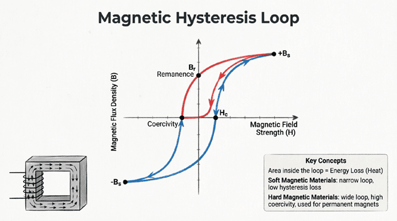
To understand hysteresis, we must examine the relationship between the magnetizing force ($H$) and the resulting magnetic flux density ($B$). This relationship is plotted on a graph known as the B-H Curve or Hysteresis Loop.

Tracing the Hysteresis Loop

Imagine starting with a completely unmagnetized piece of iron (Point O). We gradually increase the magnetizing force ($H$) by increasing the current in a surrounding coil.

1. Initial Magnetization (O to A): As $H$ increases, $B$ increases rapidly. The magnetic domains inside the iron begin to align with the external field.
2. Saturation (Point A): Eventually, nearly all magnetic domains are aligned. Further increases in $H$ produce very little increase in $B$. The material has reached magnetic saturation ($B_{sat}$).
3. Reducing H to Zero (A to B): Now, we gradually decrease the current, reducing $H$ back to zero. However, $B$ does not retrace the original path. It drops to a lower value, but it does not reach zero. The value of $B$ remaining when $H = 0$ is called Retentivity or Remanence ($B_r$). The material has become a permanent magnet.
4. Applying Reverse H (B to C): To reduce the flux density $B$ to zero, we must apply a magnetizing force in the opposite direction (negative $H$). The amount of reverse $H$ required to bring $B$ back to zero is called the Coercivity or Coercive Force ($H_c$).
5. Reverse Saturation (C to D): Continuing to increase the negative $H$ drives the material into negative saturation (Point D), where all domains are aligned in the opposite direction.
6. Completing the Loop (D to E to F to A): Reducing negative $H$ to zero leaves negative retentivity (Point E). Applying positive $H$ again brings $B$ to zero at positive coercivity (Point F), and further increasing $H$ brings the material back to positive saturation (Point A), closing the loop.

This closed, figure-eight-shaped path is the Hysteresis Loop.

What are Retentivity and Coercivity?
Retentivity (Remanence, $B_r$) is the amount of magnetic flux density remaining in a material after the external magnetizing force is reduced to zero. Coercivity (Coercive Force, $H_c$) is the amount of reverse magnetizing force required to reduce the remaining flux density back to zero.

Key Parameters of the Hysteresis Loop

The shape and size of the hysteresis loop reveal critical properties of the magnetic material:

1. Saturation Flux Density ($B_{sat}$)

The maximum magnetic flux density the material can achieve. Beyond this point, the material cannot be magnetized further, regardless of how much current is applied. For pure iron, this is typically around 2.1 to 2.2 Tesla.

2. Retentivity / Remanence ($B_r$)

Measured in Tesla (T). High retentivity is desirable for permanent magnets (so they stay strong) but undesirable for transformer cores (where we want the magnetism to disappear when the AC current crosses zero).

3. Coercivity / Coercive Force ($H_c$)

Measured in Amperes per meter (A/m) or Oersteds (Oe). It represents the material’s resistance to becoming demagnetized.

• Low $H_c$: Easy to magnetize and demagnetize (ideal for AC cores).
• High $H_c$: Hard to demagnetize (ideal for permanent magnets).

4. Permeability ($\mu$)

The slope of the B-H curve at any point represents the permeability ($\mu = B/H$). Permeability is not constant; it is highest in the linear region of the initial magnetization curve and drops to near $\mu_0$ (permeability of free space) at saturation.

Hysteresis Loss: The Cost of Magnetization

Every time a ferromagnetic material is cycled through a hysteresis loop, energy is expended. This energy is dissipated as heat and is known as Hysteresis Loss.

Physical Cause of Hysteresis Loss

At the microscopic level, ferromagnetic materials are divided into magnetic domains (tiny regions where atomic magnetic moments are aligned). When an external field is applied, domain walls move, and domains rotate to align with the field.

This movement is not perfectly smooth. Domain walls encounter impurities, grain boundaries, and crystal defects, causing “friction.” Overcoming this internal friction requires energy. When the field is reversed, more energy is expended to flip the domains back. This expended energy is converted directly into heat.

Steinmetz’s Empirical Equation

In 1892, Charles Proteus Steinmetz developed an empirical formula to calculate hysteresis power loss in magnetic cores:

$P_h = \eta \cdot f \cdot B_{max}^n \cdot V$

Where:

• $P_h$ = Hysteresis power loss in Watts (W)
• $\eta$ (eta) = Steinmetz’s hysteresis coefficient (depends on the material, typically $100$ to $500$ in SI units)
• $f$ = Frequency of magnetic reversal in Hertz (Hz)
• $B_{max}$ = Maximum flux density in Tesla (T)
• $n$ = Steinmetz exponent (typically between $1.6$ and $2.0$, often approximated as $1.6$ for silicon steel)
• $V$ = Volume of the magnetic core in cubic meters (m³)

The Area of the Loop

A fundamental principle of physics is that the area enclosed by the B-H hysteresis loop is directly proportional to the energy lost per cycle per unit volume.

• A wide loop has a large area = High hysteresis loss.
• A narrow loop has a small area = Low hysteresis loss.

What causes hysteresis loss?
Hysteresis loss is caused by the internal “friction” of magnetic domains flipping back and forth as the external magnetic field reverses direction. This friction converts electrical energy into heat. The energy lost per cycle is proportional to the area inside the B-H hysteresis loop.

Soft vs. Hard Magnetic Materials

Based on their hysteresis characteristics, ferromagnetic materials are broadly classified into two categories:

1. Soft Magnetic Materials

Characteristics:

• Narrow hysteresis loop (small area)
• Low coercivity ($H_c$): Easy to magnetize and demagnetize
• High permeability ($\mu$): Easily supports magnetic flux
• Low hysteresis loss: Minimal energy wasted as heat

Examples:

• Soft iron
• Silicon steel (electrical steel)
• Permalloy (Nickel-Iron alloy)
• Ferrites

Applications:

• Transformer cores
• Electric motor and generator stators/rotors
• Electromagnets
• Inductor cores
  (In these applications, the magnetic field reverses direction 50 or 60 times per second, so low loss is critical).

2. Hard Magnetic Materials

Characteristics:

• Wide hysteresis loop (large area)
• High coercivity ($H_c$): Very difficult to demagnetize
• High retentivity ($B_r$): Retains strong magnetism after the external field is removed
• High hysteresis loss (though this doesn’t matter for static applications)

Examples:

• Alnico (Aluminum-Nickel-Cobalt)
• Neodymium-Iron-Boron (NdFeB)
• Hardened carbon steel
• Samarium-Cobalt (SmCo)

Applications:

• Permanent magnets (speakers, motors)
• Magnetic data storage (hard disk drives, magnetic tape)
• Magnetic sensors
  (In these applications, we want the material to “remember” its magnetic state indefinitely).

Property	Soft Magnetic Materials	Hard Magnetic Materials
Hysteresis Loop	Narrow (small area)	Wide (large area)
Coercivity ($H_c$)	Low	High
Retentivity ($B_r$)	Low to Moderate	High
Permeability ($\mu$)	Very High	Moderate to Low
Primary Use	AC machines, transformers	Permanent magnets, data storage

Practical Applications of Hysteresis

While hysteresis loss is a nuisance in power systems, the hysteresis phenomenon itself is ingeniously exploited in several technologies:

1. Magnetic Data Storage

Hard disk drives (HDDs) and magnetic tapes rely entirely on hysteresis. The read/write head applies a strong, localized magnetic field to flip the domains of a tiny region on the disk (writing a 1 or 0). Because the material is “hard” (high retentivity and coercivity), the magnetic state remains stable even after the write head moves away, preserving the data.

2. Transformer and Motor Core Design

To minimize hysteresis loss, electrical engineers use soft magnetic materials like silicon steel. Adding 2-4% silicon to steel increases its electrical resistivity (reducing eddy current losses, a separate core loss) and significantly narrows the hysteresis loop, reducing hysteresis loss.

3. Magnetic Shielding

Materials with very high permeability and narrow hysteresis loops (like Mu-metal) are used to shield sensitive electronic equipment from external magnetic fields. They provide an easy path for magnetic flux lines, diverting them away from the protected area.

4. Hysteresis Motors

A specialized type of synchronous motor uses a rotor made of a material with a wide hysteresis loop. The rotating stator field drags the rotor’s magnetic domains along due to hysteresis, producing smooth, vibration-free torque without the need for DC excitation or windings on the rotor.

Practical Examples and Calculations

Example 1: Calculating Hysteresis Loss

Problem: A transformer core is made of silicon steel with a volume of $0.005 \text{ m}^3$. It operates at a frequency of $60 \text{ Hz}$ with a maximum flux density of $1.5 \text{ T}$. The Steinmetz hysteresis coefficient ($\eta$) for this material is $250$, and the exponent $n$ is $1.6$. Calculate the hysteresis power loss.

Solution:

Given:

• $V = 0.005 \text{ m}^3$
• $f = 60 \text{ Hz}$
• $B_{max} = 1.5 \text{ T}$
• $\eta = 250$
• $n = 1.6$

Formula:
$P_h = \eta \cdot f \cdot B_{max}^n \cdot V$

Step 1: Calculate $B_{max}^n$
$1.5^{1.6} \approx 1.912$

Step 2: Substitute values into the formula
$P_h = 250 \times 60 \times 1.912 \times 0.005$

Step 3: Multiply
$P_h = 15,000 \times 1.912 \times 0.005$
$P_h = 28,680 \times 0.005$
$P_h = 143.4 \text{ Watts}$

Result: The transformer core dissipates 143.4 Watts of power as heat due solely to magnetic hysteresis.

Example 2: Effect of Frequency and Flux Density on Loss

Problem: Using the transformer from Example 1, what happens to the hysteresis loss if the operating frequency is increased to $120 \text{ Hz}$ and the maximum flux density is reduced to $1.0 \text{ T}$?

Solution:

Given:

• $f_{new} = 120 \text{ Hz}$
• $B_{new} = 1.0 \text{ T}$
• Other parameters remain the same ($\eta = 250$, $n = 1.6$, $V = 0.005 \text{ m}^3$)

Calculation:
$P_{h(new)} = 250 \times 120 \times (1.0)^{1.6} \times 0.005$
$P_{h(new)} = 30,000 \times 1 \times 0.005$
$P_{h(new)} = 150 \text{ Watts}$

Analysis:
Even though the flux density was reduced (which normally reduces loss), doubling the frequency doubled the number of hysteresis cycles per second. Because $B_{max}^n$ dropped from $1.912$ to $1.0$, the net effect was a slight increase in total hysteresis loss (from 143.4 W to 150 W). This highlights why high-frequency transformers (like those in switch-mode power supplies) must use specialized ferrite cores with extremely low $\eta$ values.

Summary and Conclusion

Magnetic hysteresis is a fundamental property of ferromagnetic materials that describes the lag of magnetic flux density behind the applied magnetizing force. While it is the foundational principle that allows for permanent magnets and magnetic data storage, it is also a primary source of energy inefficiency in AC electrical machines.

Key takeaways from this guide:

1. The B-H Curve: Graphically represents the relationship between magnetizing force ($H$) and flux density ($B$), forming a closed loop when subjected to alternating fields.
2. Retentivity ($B_r$): The residual magnetism left in a material when the external field is removed.
3. Coercivity ($H_c$): The reverse magnetic field required to demagnetize the material completely.
4. Hysteresis Loss: Energy lost as heat due to internal domain friction during magnetization reversal. It is proportional to the area of the B-H loop and calculated using Steinmetz’s equation: $P_h = \eta f B_{max}^n V$.
5. Material Selection:

• Soft magnetic materials (narrow loop, low $H_c$) are used for transformer and motor cores to minimize losses.
• Hard magnetic materials (wide loop, high $H_c$) are used for permanent magnets and data storage to retain magnetism.

Understanding and managing magnetic hysteresis is a cornerstone of electrical engineering. By selecting appropriate core materials and optimizing operating flux densities, engineers can design highly efficient transformers, motors, and generators that power the modern world with minimal energy waste.