Negative Feedback Systems

Negative Feedback Systems: Complete Guide to Stabilization and Control

Introduction to Negative Feedback Systems

Negative feedback is arguably the most important concept in modern electronics system and control systems. It’s the principle that enables precise amplification, stable operation, and accurate control in countless applications—from the operational amplifier in your smartphone to the cruise control in your car, from audio amplifiers to industrial process controllers.

A negative feedback system is a system where a portion of the output signal is fed back to the input in opposite phase (180° out of phase), effectively subtracting from the input signal. This seemingly simple concept has profound implications: it trades raw gain for precision, stability, and predictability.

The power of negative feedback lies in its ability to:

• Stabilize unstable systems and prevent oscillations
• Reduce distortion and improve linearity
• Extend bandwidth and improve frequency response
• Desensitize gain to component variations
• Control impedance (input and output)
• Improve signal-to-noise ratio

Harold Black invented the negative feedback amplifier in 1927, revolutionizing telecommunications and laying the foundation for modern electronics. His insight—that sacrificing gain could yield stability and linearity—remains one of the most important principles in engineering.

This comprehensive guide will explore negative feedback systems in depth, covering fundamental principles, feedback topologies, mathematical analysis, practical design considerations, and real-world applications. Whether you’re designing a precision amplifier or studying control theory, mastering negative feedback is essential.

What is Negative Feedback?
Negative feedback is a system where the output is fed back to the input in opposite phase, reducing the overall gain but improving stability, linearity, bandwidth, and accuracy. It’s the foundation of precision amplifiers, control systems, and stable electronic circuits.

Fundamental Principles of Negative Feedback

Basic Concept and Operation

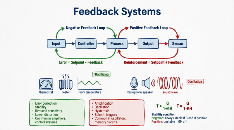
In a negative feedback system, the feedback signal opposes the input signal, creating a self-correcting mechanism. When the output increases, the feedback signal increases in the opposite direction, reducing the net input and preventing runaway conditions.

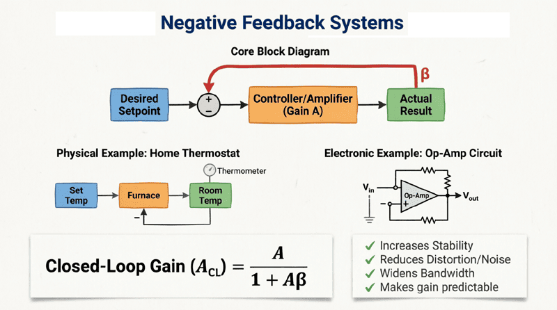
Basic Negative Feedback Loop:

Input Signal → [⊕] → [Forward Amplifier A] → Output Signal
                ↑ -                          |
                ──[Feedback Network β]←─────┘

Signal Flow:

1. Input signal enters the summing point
2. Feedback signal (β × Output) is subtracted from input
3. Error signal (difference) is amplified by forward gain A
4. Output is produced
5. Portion of output is fed back through feedback network β
6. Process repeats continuously

Mathematical Analysis

Closed-Loop Gain Derivation:

Let:

• A = Open-loop gain (forward gain)
• β = Feedback factor (0 < β < 1)
• X_i = Input signal
• X_f = Feedback signal = βX_o
• X_e = Error signal = X_i – X_f
• X_o = Output signal

Output equation:
$X_o = A \cdot X_e = A(X_i – X_f) = A(X_i – \beta X_o)$

Solving for X_o:
$X_o = AX_i – A\beta X_o$

$X_o + A\beta X_o = AX_i$

$X_o(1 + A\beta) = AX_i$

Closed-loop gain:
$A_f = \frac{X_o}{X_i} = \frac{A}{1 + A\beta}$

Where:

• A_f = Closed-loop gain (with feedback)
• A = Open-loop gain (without feedback)
• Aβ = Loop gain (product of forward and feedback gains)
• 1 + Aβ = Desensitivity factor (or return difference)

Key Parameters

Loop Gain (Aβ):
The product of forward gain and feedback factor. High loop gain provides:

• Better accuracy
• Lower distortion
• Higher desensitivity
• Wider bandwidth

Desensitivity Factor (1 + Aβ):
Measures how much feedback reduces sensitivity:

• Gain sensitivity reduced by factor (1 + Aβ)
• Distortion reduced by factor (1 + Aβ)
• Noise reduced by factor (1 + Aβ)

Feedback Factor (β):
Determined by feedback network:

• Usually resistive divider
• Sets closed-loop gain
• Should be stable and precise

Feedback Topologies

Negative feedback can be applied in four basic configurations, classified by how the feedback signal is sampled from the output and mixed with the input.

1. Voltage-Series Feedback (Series-Shunt)

Configuration:

• Sampling: Voltage sampling (shunt at output)
• Mixing: Series mixing at input
• Also called: Series-shunt feedback

Characteristics:

• Input impedance: Increases by (1 + Aβ)
• Output impedance: Decreases by (1 + Aβ)
• Gain stabilized: Voltage gain
• Ideal for: Voltage amplifiers

Circuit Example: Non-inverting op-amp amplifier

Gain Formula:
$A_f = \frac{A}{1 + A\beta} \approx \frac{1}{\beta}$ (for large Aβ)

Where $\beta = \frac{R_1}{R_1 + R_f}$

Applications:

• Voltage amplifiers
• Buffer amplifiers
• Precision amplifiers

2. Voltage-Shunt Feedback (Shunt-Shunt)

Configuration:

• Sampling: Voltage sampling (shunt at output)
• Mixing: Shunt mixing at input
• Also called: Shunt-shunt feedback

Characteristics:

• Input impedance: Decreases by (1 + Aβ)
• Output impedance: Decreases by (1 + Aβ)
• Gain stabilized: Transresistance (V/I)
• Ideal for: Transresistance amplifiers

Circuit Example: Inverting op-amp amplifier

Gain Formula:
$A_f = \frac{V_o}{I_i} \approx -R_f$ (for large loop gain)

Applications:

• Current-to-voltage converters
• Photodiode amplifiers
• Transimpedance amplifiers

3. Current-Series Feedback (Series-Series)

Configuration:

• Sampling: Current sampling (series at output)
• Mixing: Series mixing at input
• Also called: Series-series feedback

Characteristics:

• Input impedance: Increases by (1 + Aβ)
• Output impedance: Increases by (1 + Aβ)
• Gain stabilized: Transconductance (I/V)
• Ideal for: Transconductance amplifiers

Circuit Example: Common-emitter amplifier with emitter resistor

Gain Formula:
$A_f = \frac{I_o}{V_i} \approx \frac{1}{R_E}$ (for large loop gain)

Applications:

• Voltage-to-current converters
• Current sources
• Transconductance amplifiers

4. Current-Shunt Feedback (Shunt-Series)

Configuration:

• Sampling: Current sampling (series at output)
• Mixing: Shunt mixing at input
• Also called: Shunt-series feedback

Characteristics:

• Input impedance: Decreases by (1 + Aβ)
• Output impedance: Increases by (1 + Aβ)
• Gain stabilized: Current gain
• Ideal for: Current amplifiers

Circuit Example: Common-emitter amplifier with feedback resistor

Gain Formula:
$A_f = \frac{I_o}{I_i} \approx \frac{R_f}{R_E}$ (for large loop gain)

Applications:

• Current amplifiers
• Current mirrors
• Current buffers

Topology Comparison Table

Topology	Input Z	Output Z	Gain Type	Amplifier Type
Voltage-Series	Increases	Decreases	Voltage gain	Voltage amplifier
Voltage-Shunt	Decreases	Decreases	Transresistance	I-to-V converter
Current-Series	Increases	Increases	Transconductance	V-to-I converter
Current-Shunt	Decreases	Increases	Current gain	Current amplifier

Effects of Negative Feedback

1. Gain Desensitivity

Negative feedback reduces the sensitivity of gain to component variations, temperature changes, and aging.

Sensitivity Formula:

Sensitivity of closed-loop gain to changes in open-loop gain:

$S = \frac{dA_f/A_f}{dA/A} = \frac{1}{1 + A\beta}$

Interpretation:

• Without feedback (β = 0): S = 1 (100% sensitive)
• With feedback: S = 1/(1 + Aβ) (reduced sensitivity)
• Example: If Aβ = 99, sensitivity reduced by factor of 100

Practical Example:

• Op-amp open-loop gain A = 100,000
• Feedback factor β = 0.01
• Loop gain Aβ = 1,000
• Desensitivity factor = 1,001
• If A varies by 50%, A_f varies by only 0.05%

2. Bandwidth Extension

Negative feedback extends the bandwidth of amplifiers by trading gain for bandwidth.

Gain-Bandwidth Product:

For a single-pole amplifier:
$GBW = A \cdot f_H = \text{constant}$

Where:

• A = Midband gain
• f_H = Upper cutoff frequency

With Feedback:
$A_f \cdot f_{Hf} = A \cdot f_H$

Since $A_f < A$, therefore $f_{Hf} > f_H$

Bandwidth Extension Factor:
$f_{Hf} = f_H(1 + A\beta)$

Example:

• Open-loop: A = 10,000, f_H = 100 Hz
• Feedback: β = 0.01, Aβ = 100
• Closed-loop: A_f ≈ 100, f_{Hf} = 100 × 101 = 10.1 kHz
• Bandwidth increased 101 times!

3. Distortion Reduction

Negative feedback reduces nonlinear distortion by the desensitivity factor.

Distortion Reduction:

$D_f = \frac{D}{1 + A\beta}$

Where:

• D = Distortion without feedback
• D_f = Distortion with feedback

Mechanism:

• Feedback compares output with input
• Error signal contains distortion components
• Amplifier corrects for distortion
• Result: Cleaner output

Example:

• Amplifier with 10% THD (Total Harmonic Distortion)
• Loop gain Aβ = 99
• With feedback: THD = 10% / 100 = 0.1%
• 100× improvement!

4. Noise Reduction

Negative feedback can reduce noise, but the effect depends on where the noise is introduced.

Noise Analysis:

Noise at Input:

• Not reduced by feedback
• Amplified same as signal
• SNR unchanged

Noise in Amplifier:

• Reduced by factor (1 + Aβ)
• Feedback corrects for internal noise
• Improved SNR

Noise at Output:

• Not reduced by feedback
• Appears directly at output

Key Insight:
Feedback reduces noise generated within the feedback loop but not noise at the input or output.

5. Impedance Modification

Negative feedback modifies input and output impedances depending on topology.

Input Impedance:

Series mixing (voltage-series, current-series):
$Z_{if} = Z_i(1 + A\beta)$

• Input impedance increases
• Better for voltage amplifiers

Shunt mixing (voltage-shunt, current-shunt):
$Z_{if} = \frac{Z_i}{1 + A\beta}$

• Input impedance decreases
• Better for current amplifiers

Output Impedance:

Voltage sampling (voltage-series, voltage-shunt):
$Z_{of} = \frac{Z_o}{1 + A\beta}$

• Output impedance decreases
• Better voltage source

Current sampling (current-series, current-shunt):
$Z_{of} = Z_o(1 + A\beta)$

• Output impedance increases
• Better current source

6. Improved Stability

Negative feedback improves stability by:

• Reducing gain sensitivity
• Damping oscillations
• Increasing phase margin
• Preventing thermal runaway

Stability Criterion:
System is stable if loop gain Aβ doesn’t cause:

• Magnitude ≥ 1 at phase shift = 180°
• Oscillation condition avoided

Practical Design Considerations

1. Choosing Feedback Factor β

Trade-offs:

• Large β: Lower gain, better stability, wider bandwidth
• Small β: Higher gain, narrower bandwidth, less stability

Design Steps:

1. Determine required closed-loop gain A_f
2. Calculate β ≈ 1/A_f (for large loop gain)
3. Verify loop gain Aβ is sufficient (> 10 recommended)
4. Check stability margins

2. Ensuring Stability

Stability Analysis:

• Use Bode plots to analyze frequency response
• Check phase margin (> 45° recommended)
• Check gain margin (> 6 dB recommended)
• Add compensation if needed

Compensation Techniques:

• Dominant pole compensation: Add capacitor to create low-frequency pole
• Lead-lag compensation: Improve phase margin
• Miller compensation: Use Miller effect for pole splitting

3. Minimizing Loading Effects

Feedback Network Loading:

• Feedback network loads the amplifier
• Can reduce gain and affect frequency response
• Use high-impedance networks
• Buffer if necessary

Input/Output Loading:

• Consider source and load impedances
• Match topology to application
• Use appropriate buffering

4. Noise and Interference

Noise Considerations:

• Feedback reduces internal noise
• Input noise not reduced
• Use low-noise components
• Proper grounding and shielding

Interference Mitigation:

• Shield feedback network
• Keep feedback paths short
• Use differential signaling
• Filter high-frequency noise

5. Temperature Effects

Temperature Stability:

• Use temperature-stable components
• Feedback reduces temperature sensitivity
• Match temperature coefficients
• Consider thermal design

Practical Examples

Example 1: Non-Inverting Op-Amp Amplifier

Circuit:

• Op-amp with R_f = 10 kΩ, R_1 = 1 kΩ
• Voltage-series feedback

Analysis:
Feedback factor: $\beta = \frac{R_1}{R_1 + R_f} = \frac{1k}{1k + 10k} = 0.091$

Closed-loop gain: $A_f = 1 + \frac{R_f}{R_1} = 1 + \frac{10k}{1k} = 11$

Input impedance: Very high (increased by feedback)

Output impedance: Very low (decreased by feedback)

Performance:

• Precise gain of 11
• Stable operation
• Wide bandwidth
• Low distortion

Example 2: Emitter Follower (Voltage Follower)

Circuit:

• Common-collector BJT amplifier
• 100% voltage-series feedback (β = 1)

Characteristics:

• Voltage gain ≈ 1
• High input impedance
• Low output impedance
• Current gain > 1

Applications:

• Buffer amplifier
• Impedance matching
• Signal isolation

Example 3: Transimpedance Amplifier

Circuit:

• Op-amp with feedback resistor R_f
• Photodiode connected to inverting input
• Voltage-shunt feedback

Analysis:
Gain: $V_o = -I_{in} \cdot R_f$

Input impedance: Very low (virtual ground)

Output impedance: Very low

Applications:

• Photodiode amplifier
• Current-to-voltage conversion
• Optical receivers

Summary and Conclusion

Negative feedback systems are the cornerstone of modern electronics and control engineering. By sacrificing raw gain, we gain precision, stability, bandwidth, and linearity—qualities essential for high-performance systems.

Key takeaways from this comprehensive guide include:

1. Fundamental Principle: Negative feedback subtracts a portion of the output from the input, creating a self-correcting system with closed-loop gain $A_f = \frac{A}{1 + A\beta}$.
2. Four Topologies:

• Voltage-series: Increases Z_in, decreases Z_out (voltage amplifiers)
• Voltage-shunt: Decreases Z_in, decreases Z_out (I-to-V converters)
• Current-series: Increases Z_in, increases Z_out (V-to-I converters)
• Current-shunt: Decreases Z_in, increases Z_out (current amplifiers)

3. Key Benefits:

• Gain desensitivity: Reduced by factor (1 + Aβ)
• Bandwidth extension: Increased by factor (1 + Aβ)
• Distortion reduction: Reduced by factor (1 + Aβ)
• Impedance control: Tailored to application needs
• Improved stability: Prevents oscillations and runaway

4. Design Considerations:

• Choose appropriate feedback topology
• Ensure adequate loop gain (Aβ > 10)
• Verify stability margins
• Minimize loading effects
• Consider noise and temperature

5. Practical Applications:

• Operational amplifier circuits
• Audio amplifiers
• Voltage regulators
• Control systems
• Instrumentation amplifiers

Mastering negative feedback is essential for any engineer working with amplifiers, control systems, or signal processing. The principles outlined in this guide provide the foundation for designing stable, precise, and high-performance systems.

Remember: negative feedback is not just a technique—it’s a fundamental principle that enables the precision and reliability we expect from modern electronic systems. Embrace the trade-off of gain for performance, and you’ll unlock the full potential of your designs.