RC Integrator

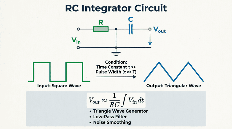
RC Integrator Circuit: Complete Guide to Integration and Waveform Conversion

Introduction to RC Integrators

An RC integrator is a fundamental analog circuit that performs the mathematical operation of integration on an input signal. When properly designed, an RC circuit can convert a square wave into a triangular wave, extract the average DC component of a signal, or smooth out rapid voltage fluctuations.

Integration is one of the most important mathematical operations in signal processing, control systems, and analog computing. In the physical world, integration represents:

• Accumulation: Adding up quantities over time
• Area under a curve: Calculating total displacement from velocity
• Smoothing: Averaging out rapid fluctuations
• Memory: Remembering past inputs

The beauty of the RC integrator is its simplicity. With just a resistor and a capacitor, you can create a circuit that performs calculus operations on electrical signals. This makes it invaluable for applications ranging from analog-to-digital converters to waveform generators and signal filters.

This comprehensive guide will explore the theory, design, and practical applications of RC integrator circuits, helping you understand when and how to use them effectively.

What is an RC Integrator?
An RC integrator is a series RC circuit where the output is taken across the capacitor. When the time constant $\tau = RC$ is much larger than the input signal’s period ($\tau \gg T$), the circuit performs mathematical integration, converting square waves to triangular waves and extracting the average value of the input signal.

The Theory of Integration in RC Circuits

Mathematical Foundation

Integration is the process of finding the area under a curve. Mathematically, the integral of a function $v_{in}(t)$ with respect to time is:

$v_{out}(t) = \frac{1}{RC} \int_0^t v_{in}(\tau) d\tau$

In an RC circuit, the capacitor voltage is related to the current by:

$i = C \frac{dv_c}{dt}$

Rearranging and integrating:

$v_c(t) = \frac{1}{C} \int i(t) dt$

Since the current through the resistor is approximately $i \approx v_{in}/R$ (when $v_c \ll v_{in}$), we get:

$v_c(t) \approx \frac{1}{RC} \int v_{in}(t) dt$

This shows that the capacitor voltage is proportional to the integral of the input voltage!

Circuit Configuration

An RC integrator consists of:

1. Resistor (R) in series with the input
2. Capacitor (C) connected to ground
3. Output taken across the capacitor

This is identical to a low-pass RC filter, but we analyze it differently—focusing on its integration properties rather than its frequency response.

The Integration Condition

For an RC circuit to act as a good integrator, it must satisfy the integration condition:

$\tau = RC \gg T$ or $\tau \gg t_p$

Where:

• $\tau$ = Time constant
• T = Period of the input signal
• $t_p$ = Pulse width of the input signal

Rule of Thumb: For good integration, $\tau$ should be at least 10 times larger than the pulse width ($\tau \ge 10 t_p$).

Why This Condition Works

When $\tau \gg t_p$:

• The capacitor charges very slowly compared to the input signal changes
• The capacitor voltage $v_c$ remains much smaller than the input voltage $v_{in}$
• The voltage across the resistor is approximately equal to the input voltage ($v_R \approx v_{in}$)
• The current is approximately $i \approx v_{in}/R$
• The capacitor integrates this current over time

If $\tau$ is too small, the capacitor charges too quickly, $v_c$ becomes significant, and the circuit no longer performs accurate integration.

When does an RC circuit act as an integrator?
An RC circuit acts as an integrator when the time constant $\tau = RC$ is much larger than the input signal period (typically $\tau \ge 10T$). Under this condition, the capacitor charges slowly, and the output voltage across the capacitor is proportional to the integral of the input voltage.

RC Integrator Response to Different Waveforms

Square Wave Input → Triangular Wave Output

This is the most common and useful application of an RC integrator.

Input: Square wave alternating between 0V and $V_{in}$
Output: Triangular wave

How it works:

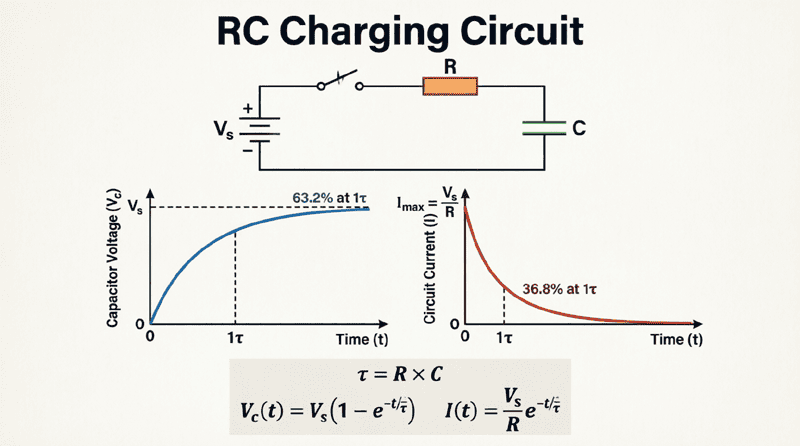
• During the high pulse ($V_{in}$), the capacitor charges linearly (approximately), creating a rising ramp
• During the low pulse (0V), the capacitor discharges linearly, creating a falling ramp
• The result is a triangular waveform

Mathematical Analysis:
For a square wave of amplitude $V_{in}$ and pulse width $t_p$:

During charging (0 to $t_p$):
$v_{out}(t) = \frac{1}{RC} \int_0^t V_{in} d\tau = \frac{V_{in}}{RC} t$

This is a linear ramp with slope $V_{in}/RC$.

Peak-to-Peak Output Voltage:
$V_{pp(out)} = \frac{V_{in} \times t_p}{RC} = \frac{V_{in} \times t_p}{\tau}$

This shows that the output amplitude is inversely proportional to the time constant!

Pulse Train Input → Staircase Output

Input: Periodic pulses (not 50% duty cycle)
Output: Staircase waveform

Each pulse adds a “step” to the output voltage. Between pulses, the capacitor discharges slightly. This creates a staircase pattern that can be used for:

• Analog-to-digital conversion
• Voltage ramp generation
• Timing circuits

Sine Wave Input → Phase-Shifted Cosine Output

Input: $v_{in}(t) = V_m \sin(\omega t)$
Output: $v_{out}(t) = -\frac{V_m}{\omega RC} \cos(\omega t)$

The integrator converts a sine wave into a cosine wave (90° phase shift) with amplitude inversely proportional to frequency. This is the basis for:

• Phase shifters
• Quadrature oscillators
• Frequency-dependent gain circuits

Triangle Wave Input → Parabolic Output

Input: Triangular wave
Output: Parabolic (quadratic) waveform

Since the integral of a linear ramp is a quadratic function, the output becomes parabolic. This demonstrates the integrator’s ability to perform successive integration operations.

Design Considerations for RC Integrators

Choosing the Time Constant

The time constant $\tau = RC$ is the most critical design parameter.

For Square Wave Integration:

• Minimum: $\tau \ge 10 t_p$ (for reasonable integration)
• Better: $\tau \ge 100 t_p$ (for excellent integration)
• Trade-off: Larger $\tau$ means smaller output amplitude

Example:
For a 1 kHz square wave ($T = 1$ ms, $t_p = 0.5$ ms):

• Minimum $\tau = 10 \times 0.5 \text{ ms} = 5 \text{ ms}$
• Better $\tau = 100 \times 0.5 \text{ ms} = 50 \text{ ms}$

Selecting R and C Values

Once you’ve chosen $\tau$, you need to select specific R and C values. Consider:

1. Capacitor Constraints:

• Available standard values
• Leakage current (use film or ceramic capacitors, avoid electrolytics for precision)
• Voltage rating (must exceed maximum output voltage)
• Physical size and cost

2. Resistor Constraints:

• Available standard values
• Power dissipation ($P = V_{in}^2/R$)
• Input impedance of the next stage (should be $\gg R$)
• Noise (larger resistors generate more thermal noise)

Typical Ranges:

• R: 1 kΩ to 1 MΩ
• C: 100 pF to 10 μF

Example Design:
For $\tau = 10$ ms:

• Option 1: R = 100 kΩ, C = 100 nF
• Option 2: R = 10 kΩ, C = 1 μF
• Option 3: R = 1 MΩ, C = 10 nF

Choose based on availability, cost, and loading requirements.

Loading Effects

The integrator output must drive the next stage of the circuit. If the load resistance $R_L$ is too small, it will discharge the capacitor and distort the integration.

Rule: $R_L \ge 10R$ (load resistance should be at least 10 times the series resistor)

If this condition cannot be met, use a voltage follower (op-amp buffer) between the integrator and the load.

Frequency Limitations

Low-Frequency Limit:
At very low frequencies, the capacitor has time to charge significantly, violating the integration condition. The circuit behaves more like a simple RC charging circuit than an integrator.

High-Frequency Limit:
At very high frequencies:

• Capacitor parasitic inductance becomes significant
• Resistor parasitic capacitance affects performance
• Op-amp limitations (if using active integrator)

Practical Range: RC integrators work best for frequencies from a few Hz to a few hundred kHz.

Practical Examples and Calculations

Example 1: Square Wave to Triangular Wave Converter

Problem: Design an RC integrator to convert a 10V, 500 Hz square wave into a triangular wave. The triangular wave should have a peak-to-peak amplitude of approximately 2V.

Solution:

Given:

• $V_{in} = 10$V
• $f = 500$ Hz
• $T = 1/500 = 2$ ms
• $t_p = T/2 = 1$ ms
• Desired $V_{pp(out)} = 2$V

Step 1: Check integration condition
For good integration: $\tau \ge 10 t_p = 10 \times 1 \text{ ms} = 10 \text{ ms}$

Step 2: Calculate required time constant from output amplitude
$V_{pp(out)} = \frac{V_{in} \times t_p}{\tau}$

$\tau = \frac{V_{in} \times t_p}{V_{pp(out)}} = \frac{10 \times 0.001}{2} = 0.005 \text{ s} = 5 \text{ ms}$

Step 3: Verify integration condition
$\tau = 5$ ms and $t_p = 1$ ms
$\tau/t_p = 5$ (This is acceptable but not excellent integration)

For better integration, we could increase $\tau$ to 10 ms, but this would reduce output amplitude to 1V.

Step 4: Choose R and C
Let’s use $\tau = 5$ ms = 0.005 s

Option: R = 50 kΩ, C = 100 nF
$\tau = 50,000 \times 100 \times 10^{-9} = 0.005$ s ✓

Result: Use R = 50 kΩ and C = 100 nF to produce a 2V triangular wave from a 10V, 500 Hz square wave.

Example 2: Pulse Integrator for ADC

Problem: A pulse train with 1V amplitude and 100 μs pulse width is applied to an RC integrator. Design the circuit to produce a staircase output where each pulse increases the output by 0.1V.

Solution:

Given:

• $V_{in} = 1$V
• $t_p = 100$ μs = $100 \times 10^{-6}$ s
• Voltage step per pulse = 0.1V

Step 1: Calculate required time constant
During each pulse: $\Delta V_{out} = \frac{V_{in} \times t_p}{\tau}$

$0.1 = \frac{1 \times 100 \times 10^{-6}}{\tau}$

$\tau = \frac{100 \times 10^{-6}}{0.1} = 1 \times 10^{-3} \text{ s} = 1 \text{ ms}$

Step 2: Verify integration condition
$\tau = 1$ ms, $t_p = 0.1$ ms
$\tau/t_p = 10$ ✓ (Good integration)

Step 3: Choose R and C
$\tau = 1$ ms = 0.001 s

Option: R = 100 kΩ, C = 10 nF
$\tau = 100,000 \times 10 \times 10^{-9} = 0.001$ s ✓

Result: Use R = 100 kΩ and C = 10 nF. Each 100 μs pulse will increase the output by 0.1V, creating a staircase waveform.

Example 3: Average Value Extraction

Problem: An RC integrator is used to extract the average (DC) value of a complex waveform with a period of 10 ms. What is the minimum time constant required?

Solution:

To extract the average value, the integrator must smooth out all variations within one period.

Rule: $\tau \ge 10T$

$\tau_{min} = 10 \times 10 \text{ ms} = 100 \text{ ms}$

Result: Use a time constant of at least 100 ms to effectively extract the DC average value.

Applications of RC Integrators

1. Waveform Generation

Triangular Wave Generators:

• Convert square waves to triangular waves
• Used in function generators
• PWM (Pulse Width Modulation) circuits

Sawtooth Generators:

• Integrate pulse trains with asymmetric duty cycles
• Used in oscilloscope timebases
• TV horizontal deflection circuits

2. Analog-to-Digital Conversion

Dual-Slope ADC:

• Integrates the input signal for a fixed time
• Then integrates a reference voltage until the output returns to zero
• The time required is proportional to the input voltage
• Highly accurate and noise-immune

3. Signal Processing

Low-Pass Filtering:

• Smooths out high-frequency noise
• Extracts DC components
• Averaging filters

Phase Shifters:

• Creates 90° phase shift for sine waves
• Used in quadrature oscillators
• Phase-locked loops

4. Control Systems

PI Controllers:

• Proportional-Integral controllers use integration
• Eliminates steady-state error
• Common in motor control and temperature control

5. Measurement Instruments

Analog Meters:

• Moving-coil meters inherently integrate
• Display average value
• Used in multimeters and panel meters

Limitations and Practical Issues

1. DC Drift

Real capacitors have leakage current, and op-amps (in active integrators) have input bias currents. These cause the output to drift over time, even with zero input.

Solution: Add a large resistor in parallel with the capacitor to provide DC feedback (creates a “leaky integrator”).

2. Saturation

If the input has a DC offset, the integrator output will ramp continuously until it hits the power supply rails (saturation).

Solution: Use AC coupling (series capacitor) at the input to block DC, or use a reset switch to periodically discharge the capacitor.

3. Limited Frequency Range

RC integrators only work well within a specific frequency range. Outside this range, the integration becomes inaccurate.

Solution: Use active integrators with op-amps for better performance, or switch to digital integration for wide frequency ranges.

4. Component Tolerances

Resistor and capacitor tolerances affect the accuracy of integration.

Solution: Use precision components (1% or better) and trim potentiometers for calibration.

Summary and Conclusion

RC integrators are elegant, simple circuits that perform the mathematical operation of integration on electrical signals. By taking the output across the capacitor in a series RC circuit with a long time constant, we can convert square waves to triangular waves, extract average values, and perform analog computation.

Key takeaways from this guide include:

1. Integration Condition: For accurate integration, $\tau = RC \ge 10 t_p$ (time constant at least 10 times the pulse width)
2. Output Relationship: $v_{out}(t) \approx \frac{1}{RC} \int v_{in}(t) dt$ (output is proportional to the integral of input)
3. Square Wave Response: Converts square waves to triangular waves with amplitude $V_{pp(out)} = \frac{V_{in} \times t_p}{\tau}$
4. Design Trade-offs: Larger $\tau$ gives better integration but smaller output amplitude
5. Applications: Waveform generation, ADCs, signal processing, control systems, and measurement instruments
6. Limitations: DC drift, saturation, limited frequency range, and component tolerances must be managed

The RC integrator is a fundamental building block in analog electronics. While modern systems often use digital signal processing or op-amp-based active integrators for better performance, understanding the passive RC integrator provides essential insight into the principles of integration, filtering, and waveform shaping. Whether you’re designing a simple tone generator or a complex control system, the RC integrator remains a valuable tool in your electrical engineering toolkit.