Closed-loop Systems
Closed-loop Systems: Complete Guide to Feedback Control Systems
Introduction to Closed-loop Systems
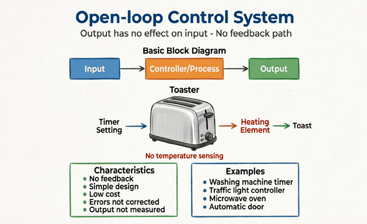
In the realm of control engineering, closed-loop systems (also known as feedback control systems) represent a sophisticated approach to achieving precise, reliable, and adaptive control. Unlike open-loop systems that operate blindly without knowledge of their output, closed-loop systems continuously monitor their performance and make real-time adjustments to achieve desired outcomes.
A closed-loop system is a control system that uses feedback to compare the actual output with the desired output, then automatically adjusts the control action to minimize the difference (error). This continuous monitoring and correction process enables closed-loop systems to maintain accuracy despite disturbances, parameter variations, and changing operating conditions.
Closed-loop systems are ubiquitous in modern technology:
- Home Appliances: Thermostats, refrigerators, washing machines with sensors
- Automotive: Cruise control, anti-lock braking systems (ABS), engine management
- Industrial: Process control, robotics, CNC machines
- Aerospace: Autopilot systems, flight control, guidance systems
- Medical: Insulin pumps, pacemakers, anesthesia machines
Understanding closed-loop systems is essential because they form the backbone of modern automation and precision control. They enable systems to:
- Maintain accuracy despite external disturbances
- Adapt to changing conditions automatically
- Compensate for component variations and aging
- Achieve higher performance than open-loop alternatives
- Ensure safety through continuous monitoring
This comprehensive guide will explore every aspect of closed-loop systems, from fundamental principles and components to design methodologies, stability analysis, and real-world applications. Whether you’re designing a temperature controller or studying advanced control theory, mastering closed-loop systems is crucial for success.
What is a Closed-loop System?
A closed-loop system is a control system that uses feedback to continuously monitor the output and compare it with the desired value, automatically adjusting the control action to minimize error. This enables precise, adaptive control despite disturbances and changing conditions.
How Closed-loop Systems Work
Fundamental Principle: Feedback
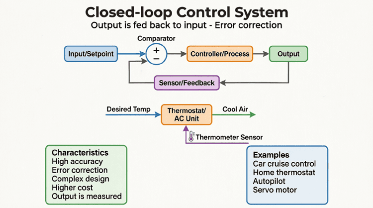
The core principle of closed-loop control is feedback—the process of measuring the system output and using that information to adjust the control action. This creates a “loop” of information flow from output back to input, hence the term “closed-loop.”
Basic Operation:
- Measure Output: Sensor measures the actual system output
- Compare with Desired: Comparator calculates the error (difference between desired and actual)
- Calculate Correction: Controller determines the appropriate control action based on error
- Apply Correction: Actuator implements the control action
- Repeat: Process continues continuously
Signal Flow in Closed-loop Systems
[Desired Output] → [Comparator] → [Controller] → [Actuator] → [Process] → [Actual Output]
                      ↑                                                              |
                      |                                                              ↓
                      └────────────────────[Sensor]←─────────────────────────────────┘
Key Elements:
- Reference Input (Setpoint):
- The desired value or target
- Example: Desired temperature = 22°C
- Sensor (Feedback Element):
- Measures actual output
- Converts physical quantity to electrical signal
- Example: Thermocouple measuring temperature
- Comparator (Summing Point):
- Calculates error: e = r – y
- Where r = reference, y = measured output
- Determines deviation from desired
- Controller:
- Processes error signal
- Generates control action
- Implements control algorithm (e.g., PID)
- Actuator:
- Executes control action
- Converts control signal to physical action
- Example: Heater, valve, motor
- Process (Plant):
- The system being controlled
- Example: Room, tank, motor
- Disturbances:
- External influences affecting the process
- Example: Drafts, load changes, ambient temperature
Mathematical Representation
For a basic closed-loop system:
Error Signal:
$e(t) = r(t) – y(t)$
Where:
- e(t) = Error signal
- r(t) = Reference input (desired value)
- y(t) = Measured output
Controller Output:
$u(t) = K \cdot e(t)$ (for proportional control)
Where:
- u(t) = Control signal
- K = Controller gain
Process Output:
$y(t) = G \cdot u(t)$
Where:
- G = Process gain
Closed-loop Transfer Function:
$\frac{Y(s)}{R(s)} = \frac{G(s)C(s)}{1 + G(s)C(s)H(s)}$
Where:
- G(s) = Process transfer function
- C(s) = Controller transfer function
- H(s) = Sensor transfer function
Example: Temperature Control System
Scenario: Maintaining room temperature at 22°C.
Components:
- Reference: Thermostat set to 22°C
- Sensor: Temperature sensor (thermistor)
- Comparator: Thermostat circuit
- Controller: ON/OFF or PID controller
- Actuator: Relay controlling heater
- Process: Room with heater
- Disturbances: Open windows, outside temperature, occupancy
Operation:
- Sensor measures actual room temperature (e.g., 20°C)
- Comparator calculates error: 22°C – 20°C = 2°C
- Controller determines heater power needed
- Relay turns ON heater
- Room temperature rises
- Sensor detects new temperature
- Process repeats continuously
Advantage: If a window opens (disturbance), the system detects temperature drop and increases heating automatically.
Key Components of Closed-loop Systems
1. Sensors (Feedback Elements)
Sensors are the eyes and ears of closed-loop systems, providing critical information about the system’s actual state.
Characteristics of Good Sensors:
Accuracy:
- How close measurement is to true value
- Example: Temperature sensor accuracy ±0.1°C
Precision:
- Repeatability of measurements
- Example: Scale giving same reading repeatedly
Sensitivity:
- Change in output per unit change in input
- High sensitivity for small changes
- Example: Microphone sensitivity
Response Time:
- Speed of measurement
- Fast response for dynamic systems
- Example: Pressure sensor response < 1ms
Linearity:
- Output proportional to input
- Simplifies calibration
- Example: Linear potentiometer
Range:
- Operating limits
- Must cover expected values
- Example: Thermometer -40°C to 150°C
Common Sensor Types:
Temperature Sensors:
- Thermocouples: Wide range, rugged
- RTDs: High accuracy, stable
- Thermistors: High sensitivity, low cost
- Infrared: Non-contact measurement
Position Sensors:
- Encoders: Digital output, high resolution
- LVDTs: Linear measurement, accurate
- Potentiometers: Simple, low cost
- Ultrasonic: Non-contact, long range
Pressure Sensors:
- Strain gauges: Versatile, reliable
- Piezoelectric: Dynamic pressure, fast
- Capacitive: High sensitivity
- Bourdon tube: Mechanical, robust
Flow Sensors:
- Turbine meters: Accurate, wide range
- Ultrasonic: Non-invasive
- Differential pressure: Simple, reliable
- Coriolis: Mass flow, accurate
2. Controllers
The controller is the brain of the closed-loop system, making decisions based on error signals.
Types of Controllers:
ON/OFF Controllers:
- Simplest type
- Two states: fully ON or fully OFF
- Example: Home thermostat
- Advantages: Simple, cheap, reliable
- Disadvantages: Oscillation around setpoint
Proportional (P) Controllers:
- Output proportional to error
- $u(t) = K_p \cdot e(t)$
- Reduces steady-state error
- May have offset
- Example: Cruise control
Proportional-Integral (PI) Controllers:
- Combines proportional and integral action
- $u(t) = K_p \cdot e(t) + K_i \int e(t) dt$
- Eliminates steady-state error
- Most common in industry
- Example: Temperature control
Proportional-Integral-Derivative (PID) Controllers:
- Combines P, I, and D actions
- $u(t) = K_p \cdot e(t) + K_i \int e(t) dt + K_d \frac{de(t)}{dt}$
- Fast response, no steady-state error
- Most versatile controller
- Example: Industrial process control
Fuzzy Logic Controllers:
- Uses linguistic rules
- Handles nonlinear systems
- Tolerates imprecision
- Example: Washing machine control
Adaptive Controllers:
- Adjusts parameters automatically
- Handles changing conditions
- Complex implementation
- Example: Aircraft control
Digital vs. Analog Controllers:
Analog Controllers:
- Continuous signal processing
- Fast response
- Simple implementation
- Example: Op-amp based PID
Digital Controllers:
- Discrete-time processing
- Flexible, programmable
- Can implement complex algorithms
- Example: Microcontroller-based control
3. Actuators
Actuators execute the control decisions, converting electrical signals into physical actions.
Types of Actuators:
Electric Actuators:
- Motors:
- DC motors: Variable speed, easy control
- AC motors: High power, industrial
- Stepper motors: Precise positioning
- Servo motors: Closed-loop control
- Solenoids:
- Linear motion
- Fast response
- Example: Valve control
- Relays:
- ON/OFF switching
- Isolation
- Example: Heater control
Pneumatic Actuators:
- Use compressed air
- Clean, fast
- Safe in explosive environments
- Example: Factory automation
Hydraulic Actuators:
- Use pressurized fluid
- High force capability
- Example: Heavy machinery
Thermal Actuators:
- Heating elements
- Coolers
- Example: Temperature control
4. Comparators
The comparator calculates the error signal by comparing reference and feedback.
Functions:
- Subtraction: e = r – y
- Signal conditioning
- Noise filtering
- Scaling
Implementation:
- Analog: Op-amp differential amplifier
- Digital: Software subtraction
- Mixed-signal: ADC + digital processing
Advantages of Closed-loop Systems
1. Error Correction
Automatic Adjustment:
- Continuously corrects for errors
- Compensates for disturbances
- Maintains accuracy
Example: Cruise control adjusts throttle when going uphill.
2. Disturbance Rejection
Handles External Influences:
- Compensates for environmental changes
- Rejects load variations
- Maintains performance
Example: Air conditioner maintains temperature despite open doors.
3. Improved Accuracy
Precise Control:
- Achieves higher accuracy than open-loop
- Reduces steady-state error
- Better tracking of setpoint
Example: CNC machine achieves micron-level precision.
4. Adaptability
Handles Changing Conditions:
- Adjusts to parameter variations
- Compensates for component aging
- Adapts to different operating points
Example: Engine control adapts to altitude changes.
5. Stability Enhancement
Controlled Response:
- Can stabilize unstable processes
- Damps oscillations
- Improves transient response
Example: Inverted pendulum stabilization.
6. Performance Optimization
Tunable Parameters:
- Adjust controller gains for optimal performance
- Balance speed vs. stability
- Minimize overshoot
Example: PID tuning for best response.
Disadvantages of Closed-loop Systems
1. Complexity
Design Complexity:
- More components (sensors, feedback circuitry)
- Complex control algorithms
- Requires expertise
Implementation Complexity:
- More wiring and connections
- Calibration required
- Testing and validation needed
2. Cost
Higher Component Cost:
- Sensors add expense
- More sophisticated controllers
- Additional circuitry
Development Cost:
- Longer design time
- More testing
- Tuning required
3. Stability Issues
Potential for Instability:
- Feedback can cause oscillations
- Requires stability analysis
- May need compensation
Example: Poorly tuned controller causes hunting.
4. Slower Response
Feedback Delay:
- Time to measure output
- Processing time
- Can limit bandwidth
Example: Slow sensor limits control speed.
5. Sensor Failures
Dependency on Sensors:
- Sensor failure causes system failure
- Requires redundancy for critical systems
- Maintenance needed
Example: Failed temperature sensor causes system shutdown.
Stability Analysis in Closed-loop Systems
What is Stability?
A stable system returns to equilibrium after a disturbance. An unstable system oscillates or diverges.
Stability Criteria:
BIBO Stability:
- Bounded Input → Bounded Output
- System doesn’t oscillate indefinitely
- Output settles to steady value
Asymptotic Stability:
- System returns to equilibrium
- No sustained oscillations
- Error goes to zero
Methods of Stability Analysis
Routh-Hurwitz Criterion:
- Algebraic method
- Determines stability without solving
- Checks characteristic equation
Root Locus:
- Graphical method
- Shows pole movement with gain
- Visualizes stability margins
Bode Plot:
- Frequency response method
- Shows gain and phase margins
- Determines stability margins
Nyquist Criterion:
- Complex plane method
- Encirclement analysis
- Comprehensive stability test
Stability Margins
Gain Margin:
- How much gain can increase before instability
- Measured in dB
- Typical: > 6 dB
Phase Margin:
- How much phase lag can increase before instability
- Measured in degrees
- Typical: > 45°
Practical Examples of Closed-loop Systems
1. Cruise Control System
Objective: Maintain constant vehicle speed.
Components:
- Reference: Driver-set speed
- Sensor: Speed sensor (wheel encoder)
- Controller: PID controller
- Actuator: Throttle actuator
- Process: Vehicle dynamics
- Disturbances: Hills, wind, load
Operation:
- Driver sets desired speed (e.g., 65 mph)
- Speed sensor measures actual speed
- Controller calculates speed error
- Adjusts throttle to minimize error
- Continuous feedback maintains speed
Advantages:
- Automatic speed maintenance
- Compensates for hills
- Improves fuel efficiency
- Reduces driver fatigue
2. Home Thermostat
Objective: Maintain room temperature.
Components:
- Reference: User-set temperature
- Sensor: Temperature sensor (thermistor/bimetal)
- Controller: ON/OFF or PID
- Actuator: Relay controlling HVAC
- Process: Room temperature
- Disturbances: Open windows, occupancy, weather
Operation:
- User sets desired temperature
- Sensor measures room temperature
- Controller compares and decides
- Turns HVAC ON/OFF
- Continuous monitoring
Types:
- Mechanical: Bimetallic strip
- Electronic: Digital sensor + microcontroller
- Smart: WiFi-enabled, programmable
3. Automatic Voltage Regulator
Objective: Maintain constant output voltage.
Components:
- Reference: Stable voltage reference
- Sensor: Voltage divider
- Controller: Error amplifier
- Actuator: Transistor/SCR
- Process: Power supply
- Disturbances: Load changes, input variations
Operation:
- Reference sets desired voltage
- Sensor measures output voltage
- Comparator calculates error
- Controller adjusts transistor
- Maintains constant output
Applications:
- Power supplies
- Generators
- Voltage stabilizers
4. Robotic Arm Position Control
Objective: Precise position control of robotic arm.
Components:
- Reference: Desired position (from program)
- Sensor: Encoder on each joint
- Controller: PID or advanced control
- Actuator: Servo motor on each joint
- Process: Robotic arm dynamics
- Disturbances: Load variations, friction
Operation:
- Program specifies desired position
- Encoders measure actual positions
- Controller calculates position errors
- Motors adjust to minimize errors
- Continuous feedback ensures accuracy
Performance:
- High precision (sub-millimeter)
- Fast response
- Handles varying loads
Design Considerations for Closed-loop Systems
1. Sensor Selection
Criteria:
- Accuracy and precision
- Response time
- Range and resolution
- Environmental compatibility
- Cost
- Reliability
Example: Temperature control needs fast, accurate sensor.
2. Controller Design
Selection:
- ON/OFF for simple applications
- P for basic proportional control
- PI for eliminating steady-state error
- PID for best overall performance
- Advanced control for complex systems
Tuning:
- Ziegler-Nichols method
- Cohen-Coon method
- Software auto-tuning
- Manual tuning
3. Stability Analysis
Methods:
- Root locus analysis
- Bode plot analysis
- Nyquist criterion
- Simulation
Margins:
- Ensure adequate gain margin (> 6 dB)
- Ensure adequate phase margin (> 45°)
- Consider robustness
4. Performance Specifications
Define Requirements:
- Rise time
- Settling time
- Overshoot
- Steady-state error
- Bandwidth
- Disturbance rejection
Example: Temperature control: ±0.5°C accuracy, < 5 min settling time.
5. Safety Considerations
Fail-Safe Design:
- Sensor failure detection
- Actuator limits
- Emergency stop
- Redundancy for critical systems
- Over-travel protection
Example: Oven with thermal cutoff even if controller fails.
6. Noise and Interference
Mitigation:
- Shielding
- Filtering
- Grounding
- Signal conditioning
- Differential measurements
Example: Low-pass filter on sensor input.
Closed-loop systems represent a sophisticated approach to control, utilizing feedback to achieve precise, adaptive, and reliable performance. By continuously monitoring the output and comparing it with the desired value, closed-loop systems can automatically correct errors, reject disturbances, and maintain accuracy under varying conditions.
Key takeaways from this comprehensive guide include:
- Fundamental Principle: Closed-loop systems use feedback to compare actual output with desired output, automatically adjusting control action to minimize error.
- Key Components:
- Sensors: Measure actual output
- Comparators: Calculate error
- Controllers: Determine control action (ON/OFF, P, PI, PID)
- Actuators: Execute control action
- Process: System being controlled
- Advantages:
- Automatic error correction
- Disturbance rejection
- Improved accuracy
- Adaptability to changing conditions
- Enhanced stability
- Performance optimization
- Disadvantages:
- Increased complexity
- Higher cost
- Potential stability issues
- Slower response due to feedback
- Dependency on sensors
- Stability Analysis:
- Critical for proper operation
- Methods: Routh-Hurwitz, Root Locus, Bode, Nyquist
- Gain and phase margins essential
- Practical Applications:
- Cruise control in vehicles
- Home thermostats
- Automatic voltage regulators
- Robotic arm control
- Industrial process control
- Design Considerations:
- Careful sensor selection
- Appropriate controller design and tuning
- Stability analysis
- Performance specifications
- Safety mechanisms
- Noise mitigation
Understanding closed-loop systems is fundamental to modern control engineering. They enable the precise, reliable, and adaptive control that modern technology demands. From simple home appliances to complex industrial automation and aerospace systems, closed-loop control is the backbone of precision automation.
As you continue your journey in control systems engineering, remember that the key to successful closed-loop design lies in understanding the trade-offs between performance, stability, complexity, and cost. Master these principles, and you’ll be well-equipped to design robust, efficient control systems for any application.