RC Waveforms

RC Waveforms: Complete Guide to Square Wave Response and Time Constants

Introduction to RC Waveforms

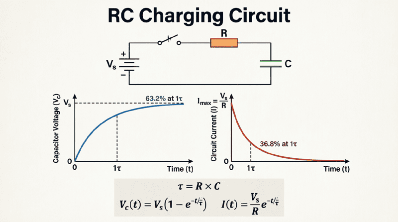
In the previous articles, we explored how an RC circuit behaves when a DC voltage is suddenly applied (charging) or removed (discharging). But what happens when we continuously switch the voltage on and off? This is where RC waveforms come into play.

When a time-varying signal, such as a square wave, is applied to an RC circuit, the capacitor undergoes continuous cycles of charging and discharging. The resulting output waveform—whether measured across the capacitor or the resistor—depends entirely on the relationship between the circuit’s time constant ($\tau$) and the pulse width ($t_p$) of the input signal.

Understanding RC waveforms is crucial for:

• Waveform shaping: Converting square waves into triangular waves or sharp spikes.
• Signal coupling: Passing AC signals while blocking DC components.
• Filtering: Designing basic high-pass and low-pass filters.
• Timing and pulse generation: Creating precise delays and trigger signals in digital electronics.

This comprehensive guide will explore how RC circuits respond to square wave inputs, breaking down the three fundamental time constant conditions and explaining how to predict and control the output waveforms.

What are RC Waveforms?
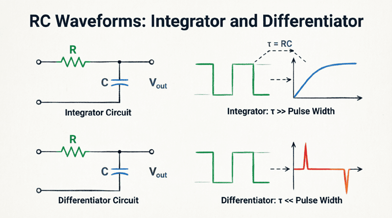
RC waveforms are the output voltage shapes produced when a time-varying input (like a square wave) is applied to an RC circuit. The shape of the output depends on the ratio of the circuit’s time constant ($\tau = RC$) to the input signal’s pulse width ($t_p$). By adjusting R or C, an RC circuit can shape a square wave into a rounded wave, a triangular wave, or sharp spikes.

The Square Wave Input

To analyze RC waveforms systematically, engineers use a square wave as the input signal. A square wave is an ideal test signal because it consists of instantaneous transitions between a high voltage ($V_{in}$) and a low voltage (0V), forcing the capacitor to continuously charge and discharge.

Key Parameters of a Square Wave

• Period ($T$): The total time for one complete cycle (high + low).
• Pulse Width ($t_p$): The duration the signal stays at the high voltage. For a standard 50% duty cycle square wave, $t_p = T / 2$.
• Frequency ($f$): The number of cycles per second, $f = 1 / T$.

When this square wave is applied to a series RC circuit, the capacitor attempts to charge toward $V_{in}$ during the high pulse, and discharge toward 0V during the low pulse. The extent to which it succeeds depends on the time constant $\tau$.

The Three Key RC Waveform Conditions

The behavior of an RC circuit driven by a square wave is categorized into three distinct conditions based on the ratio of the time constant ($\tau$) to the pulse width ($t_p$).

Condition 1: Short Time Constant ($\tau \ll t_p$)

Definition: The time constant is much smaller than the pulse width (typically $\tau < 0.1 t_p$).

Behavior:
Because $\tau$ is very small, the capacitor charges and discharges very quickly. It reaches its full steady-state voltage long before the pulse ends.

• During the high pulse, $V_c$ rapidly rises to $V_{in}$ and stays flat.
• During the low pulse, $V_c$ rapidly drops to 0V and stays flat.

Output Waveform ($V_c$):
The voltage across the capacitor looks almost exactly like the input square wave, but with slightly rounded corners (the exponential rise and fall curves are visible only at the very beginning of each pulse).

Output Waveform ($V_r$):
The voltage across the resistor consists of sharp, narrow spikes at the transitions. When the input jumps high, $V_r$ spikes to $V_{in}$ and immediately decays to zero as the capacitor charges.

Applications:

• AC Coupling / DC Blocking: Because the capacitor charges so quickly, it blocks the DC component of the signal while passing the AC transitions.
• Edge Detection: The sharp spikes across the resistor can be used to trigger digital logic circuits.

Condition 2: Medium Time Constant ($\tau \approx t_p$)

Definition: The time constant is roughly equal to the pulse width (typically $0.1 t_p < \tau < 10 t_p$).

Behavior:
The capacitor charges and discharges at a moderate rate. It does not have enough time to reach full charge before the pulse ends, nor does it fully discharge before the next pulse begins.

• During the high pulse, $V_c$ rises exponentially but only reaches a fraction of $V_{in}$.
• During the low pulse, $V_c$ falls exponentially but only drops part of the way to 0V.

Output Waveform ($V_c$):
The voltage across the capacitor forms a triangular or sawtooth-like waveform. The exponential curves blend together to create a linear-looking ramp up and ramp down.

Output Waveform ($V_r$):
The voltage across the resistor also forms a triangular waveform, but it is inverted relative to the capacitor voltage (since $V_r = V_{in} – V_c$).

Applications:

• Waveform Shaping: Converting square waves into triangular waves for function generators or modulation circuits.
• Integrator/Differentiator basics: Operating in the transition region between pure integration and differentiation.

Condition 3: Long Time Constant ($\tau \gg t_p$)

Definition: The time constant is much larger than the pulse width (typically $\tau > 10 t_p$).

Behavior:
The capacitor charges and discharges very slowly. During the brief pulse width, the capacitor only accumulates a tiny amount of charge.

• During the high pulse, $V_c$ rises only a tiny fraction of the way toward $V_{in}$.
• During the low pulse, $V_c$ drops only a tiny fraction back toward 0V.

Output Waveform ($V_c$):
The voltage across the capacitor looks like a small ripple centered around the average DC value of the input (which is $V_{in} / 2$ for a 50% duty cycle square wave). It looks almost like a straight, slightly wavy line.

Output Waveform ($V_r$):
The voltage across the resistor looks almost exactly like the input square wave, but with a slight “tilt” or “droop” on the flat tops and bottoms.

Applications:

• Low-Pass Filtering: The capacitor smooths out the square wave, extracting its average DC value.
• Power Supply Filtering: Smoothing out ripple in rectified AC signals.

How does the time constant affect RC waveforms?
If $\tau$ is short compared to the pulse width, the capacitor charges fully, producing a rounded square wave across the capacitor and sharp spikes across the resistor. If $\tau$ is medium, it produces a triangular wave. If $\tau$ is long, the capacitor barely charges, producing a small ripple across the capacitor and a tilted square wave across the resistor.

Capacitor Voltage ($V_c$) vs. Resistor Voltage ($V_r$)

It is vital to remember that in a series RC circuit, the input voltage is split between the capacitor and the resistor according to Kirchhoff’s Voltage Law:

$V_{in}(t) = V_c(t) + V_r(t)$

Because of this relationship, the waveforms across the capacitor and the resistor are complementary. If you know the shape of $V_c$, you can easily determine $V_r$ by subtracting $V_c$ from the input square wave.

• When $V_c$ is rising (charging), $V_r$ is falling.
• When $V_c$ is falling (discharging), $V_r$ is rising (in the negative direction or dropping from the peak).
• The sum of their instantaneous values always equals the input voltage at that exact moment.

Practical Examples and Calculations

Example 1: Designing a Waveform Shaper

Problem: You need to convert a 1 kHz square wave into a triangular wave using an RC circuit. The capacitor value is fixed at 10 nF. What resistor value should you choose?

Solution:

Step 1: Determine the pulse width ($t_p$).
Frequency $f = 1000$ Hz.
Period $T = 1 / f = 1 / 1000 = 1$ ms.
For a 50% duty cycle square wave, $t_p = T / 2 = 0.5$ ms.

Step 2: Choose the appropriate time constant.
To get a good triangular wave, we need a medium time constant where $\tau \approx t_p$.
Let’s choose $\tau = 0.5$ ms = $0.5 \times 10^{-3}$ s.

Step 3: Calculate the resistance.
$\tau = R \times C$
$R = \tau / C = (0.5 \times 10^{-3}) / (10 \times 10^{-9})$
$R = 50,000 \Omega = 50 \text{ k}\Omega$

Result: Use a 50 kΩ resistor with the 10 nF capacitor to produce a triangular waveform from a 1 kHz square wave.

Example 2: Designing a Coupling Circuit

Problem: An audio signal (square wave approximation) has a lowest frequency of 20 Hz. You need to design an RC coupling circuit to pass this signal while blocking DC. The load resistance is 10 kΩ. What is the maximum capacitance you should use to ensure a “short time constant”?

Solution:

Step 1: Determine the pulse width of the lowest frequency.
Lowest frequency $f = 20$ Hz.
Period $T = 1 / 20 = 50$ ms.
Pulse width $t_p = T / 2 = 25$ ms.

Step 2: Define “short time constant”.
For a coupling circuit, we want $\tau \le 0.1 t_p$.
$\tau_{max} = 0.1 \times 25 \text{ ms} = 2.5 \text{ ms} = 0.0025 \text{ s}$.

Step 3: Calculate the maximum capacitance.
$\tau = R \times C$
$C_{max} = \tau_{max} / R = 0.0025 / 10,000$
$C_{max} = 0.25 \times 10^{-6} \text{ F} = 0.25 \text{ \mu F}$

Result: Use a capacitor of 0.25 μF or smaller to ensure the circuit acts as a proper AC coupler for frequencies down to 20 Hz.

Response to Other Waveforms

While the square wave is the standard for analyzing RC transient responses, RC circuits also shape other waveforms in predictable ways:

Triangular Wave Input

When a triangular wave is applied to an RC circuit with a long time constant ($\tau \gg t_p$), the output across the capacitor becomes a parabolic waveform. The exponential charging curve smooths out the sharp peaks and valleys of the triangle, creating a curved, parabolic shape.

Sine Wave Input

When a sine wave is applied, the output remains a sine wave of the exact same frequency. However, the RC circuit alters its amplitude and phase.

• At low frequencies, the capacitor voltage ($V_c$) is nearly equal to the input, and the phase shift is near 0°.
• At high frequencies, $V_c$ drops significantly, and the phase shift approaches -90°.
  This frequency-dependent behavior is the foundation of RC filters, which we will explore in depth in future articles.

Summary and Conclusion

RC waveforms demonstrate the dynamic, time-dependent nature of capacitors and resistors. By applying a square wave and observing the output, we can visually and mathematically understand how the time constant ($\tau$) dictates circuit behavior.

Key takeaways from this guide include:

1. Square Wave Testing: Square waves are the ideal input for analyzing RC transient responses because they force continuous, predictable charging and discharging cycles.
2. Short Time Constant ($\tau \ll t_p$): Capacitor charges fully. Output across C is a rounded square wave; output across R is sharp spikes. Used for AC coupling and edge detection.
3. Medium Time Constant ($\tau \approx t_p$): Capacitor charges partially. Output across C is a triangular wave. Used for waveform shaping.
4. Long Time Constant ($\tau \gg t_p$): Capacitor charges minimally. Output across C is a small ripple; output across R is a tilted square wave. Used for low-pass filtering and smoothing.
5. Complementary Voltages: $V_c(t) + V_r(t) = V_{in}(t)$. The waveforms across the capacitor and resistor are always mathematical complements of each other.

Mastering RC waveforms allows you to intentionally shape electrical signals, design effective filters, and troubleshoot timing issues in digital and analog circuits. Whether you are building a simple tone control or a complex pulse generator, understanding the relationship between $\tau$ and $t_p$ is an indispensable skill.