Tau – The Time Constant
Tau (τ) – The RC Time Constant: Complete Guide to RC Circuit Response Time
Introduction to the Time Constant
In the world of RC circuits, one parameter reigns supreme: Tau (τ), the time constant. This single value determines how quickly a capacitor charges or discharges, how fast a circuit responds to changes, and whether an RC circuit acts as an integrator or differentiator.
The time constant is more than just a number—it’s the heartbeat of RC circuits. It tells you:
- How long it takes to charge a capacitor to 63.2% of the supply voltage
- How quickly a circuit responds to sudden changes
- Whether a filter will pass or block certain frequencies
- How long a timing circuit will delay
Understanding tau is essential for designing:
- Timing circuits: Delays, oscillators, and pulse generators
- Filters: Low-pass and high-pass filters
- Coupling circuits: AC coupling and DC blocking
- Waveform shapers: Integrators and differentiators
- Power supplies: Smoothing and filtering
This comprehensive guide will explore every aspect of the time constant, from its mathematical definition to practical measurement techniques and real-world applications.
What is the Time Constant (τ)?
The time constant τ (tau) is the product of resistance and capacitance in an RC circuit: τ = RC. It represents the time required for a capacitor to charge to 63.2% of the supply voltage or discharge to 36.8% of its initial voltage. It determines the speed of the circuit’s response to changes.
Mathematical Definition of Tau
The Fundamental Equation
The time constant is defined by a simple equation:
$\tau = R \times C$
Where:
- τ (tau) = Time constant (seconds)
- R = Resistance (ohms, Ω)
- C = Capacitance (farads, F)
This deceptively simple equation contains profound implications for circuit behavior.
Units and Dimensions
Let’s verify that τ indeed has units of time:
$\tau = R \times C = \Omega \times F$
Since:
- $\Omega = V/A$ (volts per ampere)
- $F = C/V$ (coulombs per volt)
Therefore:
$\tau = \frac{V}{A} \times \frac{C}{V} = \frac{C}{A} = \frac{C}{C/s} = s$ (seconds) ✓
The units work out perfectly—tau is indeed a time!
Physical Interpretation
The time constant represents the characteristic time scale of an RC circuit. It’s the time it takes for the circuit to respond significantly to a change.
During Charging:
After one time constant (t = τ), the capacitor voltage reaches:
$V_c = V_s(1 – e^{-1}) = V_s(1 – 0.368) = 0.632V_s$
During Discharging:
After one time constant (t = τ), the capacitor voltage drops to:
$V_c = V_0 e^{-1} = 0.368V_0$
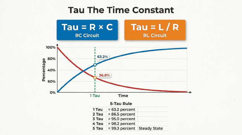
This 63.2%/36.8% relationship is universal for all first-order RC circuits!
Why is 63.2% special?
After one time constant, a charging capacitor reaches 63.2% of the final voltage because $1 – e^{-1} \approx 0.632$. This is a fundamental property of exponential growth and decay, appearing in all first-order systems.
The Significance of Tau in Circuit Behavior
Charging and Discharging Progress
The time constant provides a convenient way to estimate charging and discharging progress:
| Time Elapsed | % Charged | % Discharged | Status |
|---|---|---|---|
| t = 0 | 0% | 100% | Start |
| t = τ | 63.2% | 36.8% | One time constant |
| t = 2τ | 86.5% | 13.5% | |
| t = 3τ | 95.0% | 5.0% | |
| t = 4τ | 98.2% | 1.8% | |
| t = 5τ | 99.3% | 0.7% | Essentially complete |
The 5τ Rule:
After 5 time constants, the circuit is considered to have reached steady state (99.3% complete). This is a universal rule of thumb in circuit analysis.
Response Speed Classification
The magnitude of τ determines whether a circuit is “fast” or “slow”:
Fast Circuits (Small τ):
- τ < 1 μs: High-speed digital circuits
- τ < 1 ms: Audio frequency circuits
- Quick response to changes
- Wide bandwidth
Slow Circuits (Large τ):
- τ > 1 s: Timing and delay circuits
- τ > 1 minute: Long-term averaging
- Slow response to changes
- Narrow bandwidth
Relationship to Frequency Response
The time constant determines the cutoff frequency of an RC filter:
$f_c = \frac{1}{2\pi\tau} = \frac{1}{2\pi RC}$
Where:
- $f_c$ = Cutoff frequency (Hz)
- τ = Time constant (seconds)
At the cutoff frequency:
- The output amplitude is 70.7% of the input (-3 dB)
- The phase shift is 45°
- The circuit begins to significantly attenuate signals
Example:
For τ = 1 ms:
$f_c = \frac{1}{2\pi \times 0.001} = 159 \text{ Hz}$
This RC circuit will pass frequencies below 159 Hz and attenuate frequencies above 159 Hz.
Calculating Tau in Practical Circuits
Simple Series RC Circuit
For a simple series RC circuit:
$\tau = R_{total} \times C_{total}$
Example:
R = 10 kΩ, C = 100 nF
$\tau = 10,000 \times 100 \times 10^{-9} = 0.001 \text{ s} = 1 \text{ ms}$
Complex Circuits with Multiple Resistors
When multiple resistors are present, you must find the equivalent resistance seen by the capacitor.
Method:
- Remove the capacitor from the circuit
- Find the equivalent resistance looking into the terminals where the capacitor was connected
- Use Thevenin’s theorem if necessary
- Calculate $\tau = R_{eq} \times C$
Example:
Two resistors in parallel: R₁ = 10 kΩ, R₂ = 20 kΩ
$R_{eq} = \frac{R_1 \times R_2}{R_1 + R_2} = \frac{10k \times 20k}{10k + 20k} = 6.67 \text{ k}\Omega$
With C = 100 nF:
$\tau = 6,670 \times 100 \times 10^{-9} = 0.667 \text{ ms}$
Complex Circuits with Multiple Capacitors
When multiple capacitors are present:
Capacitors in Series:
$\frac{1}{C_{eq}} = \frac{1}{C_1} + \frac{1}{C_2} + …$
Capacitors in Parallel:
$C_{eq} = C_1 + C_2 + …$
Then: $\tau = R \times C_{eq}$
Circuits with Switches
In circuits with switches, the time constant may change depending on the switch position.
Example:
- Switch position A: τ₁ = R₁C
- Switch position B: τ₂ = R₂C
Always calculate τ for the specific circuit configuration you’re analyzing!
Measuring the Time Constant
Method 1: Oscilloscope Measurement
The most accurate method uses an oscilloscope:
Procedure:
- Apply a square wave to the RC circuit
- Observe the capacitor voltage waveform
- Measure the time to reach 63.2% of the final value
- This time equals τ
Advantages:
- Direct measurement
- Visual verification
- Accounts for parasitic effects
Equipment Needed:
- Oscilloscope
- Function generator (square wave output)
- RC circuit under test
Method 2: Multimeter Timing
For slower circuits (τ > 1 second):
Procedure:
- Apply DC voltage to the RC circuit
- Start a stopwatch when voltage is applied
- Monitor capacitor voltage with a multimeter
- Stop the stopwatch when voltage reaches 63.2% of supply
- The elapsed time equals τ
Advantages:
- Simple equipment
- Good for educational purposes
Limitations:
- Only works for slow circuits
- Less accurate than oscilloscope
- Human reaction time affects accuracy
Method 3: Calculation from Component Values
When component values are known:
Procedure:
- Measure or verify R and C values
- Calculate $\tau = R \times C$
- Account for component tolerances
Example:
R = 10 kΩ ±5%, C = 100 nF ±10%
Nominal: $\tau = 10,000 \times 100 \times 10^{-9} = 1 \text{ ms}$
Range: $\tau_{min} = 9,500 \times 90 \times 10^{-9} = 0.855 \text{ ms}$
$\tau_{max} = 10,500 \times 110 \times 10^{-9} = 1.155 \text{ ms}$
Result: τ = 1.0 ms ±15%
Practical Examples and Calculations
Example 1: Camera Flash Timing
Problem: A camera flash circuit uses a 1000 μF capacitor charged through a 10 kΩ resistor from a 300V supply. How long does it take to charge to 95% (ready to flash)?
Solution:
Step 1: Calculate time constant
$\tau = R \times C = 10,000 \times 1000 \times 10^{-6} = 10 \text{ s}$
Step 2: Determine time to reach 95%
From the charging table, 95% is reached at t = 3τ
$t_{95\%} = 3\tau = 3 \times 10 = 30 \text{ seconds}$
Result: The flash takes 30 seconds to charge to 95% readiness.
Example 2: RC Filter Design
Problem: Design an RC low-pass filter with a cutoff frequency of 1 kHz. If you use a 10 nF capacitor, what resistor value is needed, and what is the time constant?
Solution:
Step 1: Calculate required time constant from cutoff frequency
$f_c = \frac{1}{2\pi\tau}$
$\tau = \frac{1}{2\pi f_c} = \frac{1}{2\pi \times 1000} = 1.59 \times 10^{-4} \text{ s} = 159 \text{ μs}$
Step 2: Calculate resistor value
$\tau = R \times C$
$R = \frac{\tau}{C} = \frac{159 \times 10^{-6}}{10 \times 10^{-9}} = 15,900 \Omega = 15.9 \text{ k}\Omega$
Use standard value: R = 16 kΩ
Step 3: Verify
$\tau = 16,000 \times 10 \times 10^{-9} = 160 \text{ μs}$
$f_c = \frac{1}{2\pi \times 160 \times 10^{-6}} = 995 \text{ Hz}$ ✓ (close to 1 kHz)
Result: Use R = 16 kΩ and C = 10 nF for τ = 160 μs and $f_c$ ≈ 1 kHz.
Example 3: Pulse Width Measurement
Problem: An RC differentiator with τ = 10 μs is used to measure the rise time of a pulse. If the output spike has a width of 30 μs at half-maximum, estimate the input pulse rise time.
Solution:
For a differentiator, the output spike width is approximately equal to the input rise time when τ is small.
However, with τ = 10 μs, there’s some distortion.
Approximate relationship:
$t_{spike} \approx \sqrt{t_r^2 + \tau^2}$
Where:
- $t_{spike}$ = Output spike width
- $t_r$ = Input rise time
- τ = Time constant
Solving for $t_r$:
$30^2 = t_r^2 + 10^2$
$900 = t_r^2 + 100$
$t_r^2 = 800$
$t_r = 28.3 \text{ μs}$
Result: The input pulse rise time is approximately 28 μs.
Applications of Time Constant
1. Timing Circuits
Delay Circuits:
- Use τ to create precise time delays
- Example: τ = 1 s creates a 1-second delay
- Applications: Timers, oscillators, pulse generators
Monostable Multivibrators:
- One-shot pulse generators
- Pulse width determined by τ
- Applications: Debouncing switches, timing events
2. Filtering
Low-Pass Filters:
- Pass frequencies below $f_c = 1/(2\pi\tau)$
- Attenuate high frequencies
- Applications: Noise reduction, audio filtering
High-Pass Filters:
- Pass frequencies above $f_c$
- Block DC and low frequencies
- Applications: AC coupling, removing drift
3. Waveform Shaping
Integrators:
- Require τ ≫ pulse width
- Convert square waves to triangular waves
- Applications: ADC, signal averaging
Differentiators:
- Require τ ≪ rise time
- Detect edges and sharp transitions
- Applications: Edge detection, pulse sharpening
4. Power Supply Design
Smoothing Capacitors:
- Large τ reduces ripple voltage
- τ determines discharge between cycles
- Applications: DC power supplies, rectifiers
Inrush Current Limiting:
- RC circuits limit startup current
- τ determines charging rate
- Applications: Motor starting, capacitor charging
5. Signal Processing
Sample and Hold:
- τ determines acquisition time
- Must be fast enough to track input
- Applications: ADC, signal processing
Peak Detectors:
- τ determines discharge rate
- Must be slow enough to hold peak
- Applications: AM demodulation, signal monitoring
Common Mistakes and Troubleshooting
Mistake 1: Ignoring Component Tolerances
Problem: Assuming τ is exact when R and C have tolerances.
Solution: Calculate worst-case τ:
- $\tau_{min} = R_{min} \times C_{min}$
- $\tau_{max} = R_{max} \times C_{max}$
- Design for the range, not just nominal value
Mistake 2: Forgetting Parasitic Effects
Problem: Ignoring parasitic capacitance and inductance.
Solution:
- Use appropriate component types for frequency range
- Keep leads short
- Account for PCB trace capacitance
- Use simulation to verify
Mistake 3: Loading Effects
Problem: The next stage loads the RC circuit, changing the effective τ.
Solution:
- Ensure load resistance ≫ R
- Use a buffer (voltage follower)
- Recalculate τ with loading included
Troubleshooting Tips
Circuit responds too slowly:
- Check if τ is too large
- Verify R and C values
- Check for unexpected parallel resistance
Circuit responds too quickly:
- Check if τ is too small
- Verify component values
- Check for parasitic capacitance
Unexpected waveform shape:
- Verify τ relative to signal period
- Check for loading effects
- Look for parasitic elements
The time constant τ is the fundamental parameter that governs RC circuit behavior. It determines how quickly circuits respond, how filters attenuate signals, and how timing circuits operate.
Key takeaways from this guide include:
- Definition: $\tau = R \times C$ (seconds), where R is in ohms and C is in farads
- Physical Meaning: Time to charge to 63.2% or discharge to 36.8% of initial value
- The 5τ Rule: After 5 time constants, the circuit reaches 99.3% of final value and is considered at steady state
- Frequency Response: Cutoff frequency $f_c = 1/(2\pi\tau)$ determines filter characteristics
- Design Applications: Timing circuits, filters, waveform shapers, power supplies, and signal processing all rely on proper τ selection
- Measurement: Can be measured directly with an oscilloscope or calculated from component values
- Practical Considerations: Component tolerances, parasitic effects, and loading must be accounted for in real designs
Understanding tau is essential for anyone working with RC circuits. Whether you’re designing a simple delay circuit, creating an audio filter, or building a complex signal processing system, the time constant is your primary tool for controlling circuit behavior. Master this concept, and you’ll have the power to shape electrical signals with precision and confidence.