LC Oscillator Basics

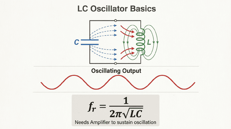
LC Oscillator Basics: Complete Guide to Tank Circuits and Oscillation Principles

Introduction to LC Oscillators

LC oscillators form the backbone of radio frequency (RF) generation, serving as the heart of countless electronic systems from radio transmitters to clock circuits. At their core, LC oscillators utilize the natural resonance between an inductor (L) and a capacitor (C) to generate continuous sinusoidal waveforms at specific frequencies.

Understanding LC oscillators is essential for anyone working with:

• Radio frequency (RF) circuits and communications
• Signal generation and test equipment
• Clock circuits in digital systems
• Wireless transmitters and receivers
• Frequency synthesis and modulation

Unlike RC oscillators that operate at lower frequencies, LC oscillators excel in the RF range (typically 100 kHz to several hundred MHz), making them indispensable in modern wireless communications, broadcasting, and high-frequency applications.

This comprehensive guide will explore the fundamental principles of LC oscillators, from the physics of tank circuits to practical design considerations, providing you with the knowledge to understand, analyze, and design these critical circuits.

What is an LC Oscillator?
An LC oscillator is an electronic circuit that uses an inductor (L) and capacitor (C) in a resonant tank circuit to generate continuous sinusoidal oscillations at a specific frequency determined by f = 1/(2π√LC). It requires an amplifying device and positive feedback to sustain oscillations.

The Physics of LC Tank Circuits

Energy Exchange in Resonant Circuits

The fundamental principle behind LC oscillators is the resonant tank circuit, which consists of an inductor and capacitor connected together. This circuit exhibits a remarkable property: it can store and exchange energy between magnetic and electric fields.

How Energy Oscillates:

1. Initial State: The capacitor is charged, storing energy in its electric field: $E = \frac{1}{2}CV^2$
2. Discharge Phase: When connected to the inductor, the capacitor discharges, creating current flow through the inductor
3. Magnetic Field Build-up: Current through the inductor creates a magnetic field, storing energy: $E = \frac{1}{2}LI^2$
4. Field Collapse: When the capacitor is fully discharged, the magnetic field collapses, inducing current that recharges the capacitor with opposite polarity
5. Reverse Cycle: The process repeats in the opposite direction, creating continuous oscillation

This energy exchange is analogous to a mass-spring system in mechanics, where energy oscillates between kinetic energy (mass motion) and potential energy (spring compression).

Natural Resonant Frequency

Every LC circuit has a natural resonant frequency at which it prefers to oscillate. This frequency is determined solely by the values of inductance and capacitance:

$f_r = \frac{1}{2\pi\sqrt{LC}}$

Where:

• $f_r$ = Resonant frequency in Hertz (Hz)
• $L$ = Inductance in Henrys (H)
• $C$ = Capacitance in Farads (F)
• $\pi$ = Pi (approximately 3.14159)

Angular Frequency:
$\omega_r = \frac{1}{\sqrt{LC}}$ (in radians per second)

Example Calculation:
For L = 10 μH and C = 100 pF:
$f_r = \frac{1}{2\pi\sqrt{10 \times 10^{-6} \times 100 \times 10^{-12}}}$
$f_r = \frac{1}{2\pi\sqrt{1 \times 10^{-15}}}$
$f_r = \frac{1}{2\pi \times 3.16 \times 10^{-8}}$
$f_r = 5.03 \text{ MHz}$

Quality Factor (Q) and Bandwidth

The Quality Factor (Q) of an LC tank circuit indicates how efficiently it stores energy and how selective it is at resonance:

$Q = \frac{f_r}{BW} = \frac{1}{R}\sqrt{\frac{L}{C}} = \frac{\omega_r L}{R} = \frac{1}{\omega_r RC}$

Where:

• BW = Bandwidth at -3dB points
• R = Equivalent series resistance (losses)

High Q Characteristics:

• Narrow bandwidth (sharp resonance)
• Low energy loss
• Better frequency stability
• Slower oscillation decay

Low Q Characteristics:

• Wide bandwidth (broad resonance)
• Higher energy loss
• Poor frequency selectivity
• Faster oscillation decay

Typical LC tank circuits have Q values ranging from 10 to several hundred, depending on component quality and circuit design.

How do you calculate the resonant frequency of an LC circuit?
The resonant frequency is calculated using: f_r = 1/(2π√LC), where L is inductance in Henrys and C is capacitance in Farads. For example, a 10μH inductor with 100pF capacitor resonates at approximately 5.03 MHz.

Barkhausen Criterion for Oscillation

For an LC circuit to function as a sustained oscillator (rather than a damped resonator), it must meet the Barkhausen Criterion, which establishes the conditions necessary for continuous oscillation.

The Two Conditions

1. Loop Gain Condition:
The total gain around the feedback loop must equal unity (1) or be slightly greater:

$|A\beta| \geq 1$

Where:

• A = Amplifier gain
• β = Feedback factor (fraction of output fed back)

Practical Consideration: Initially, $|A\beta|$ should be slightly greater than 1 to start oscillations, then stabilize at exactly 1 to maintain constant amplitude.

2. Phase Shift Condition:
The total phase shift around the loop must be 0° or a multiple of 360°:

$\angle A\beta = 0°, 360°, 720°, …$

This ensures positive (regenerative) feedback, where the feedback signal reinforces the input signal.

How It Works in LC Oscillators

In an LC oscillator:

1. The LC tank circuit provides frequency selectivity and 180° phase shift at resonance
2. The amplifier provides gain and another 180° phase shift (in common-emitter/common-source configurations)
3. Total phase shift = 180° + 180° = 360° (equivalent to 0°)
4. The feedback network returns a portion of the output to the input in phase

Starting Oscillations:

• Random noise or power-on transients provide initial signal
• Signal at resonant frequency is amplified and fed back
• Amplitude builds up with each cycle
• Non-linear effects (saturation, automatic gain control) limit amplitude
• Stable oscillation is achieved

Basic LC Oscillator Configurations

LC oscillators can be classified based on their feedback network topology. The three fundamental configurations are:

1. Tuned-Base/Tuned-Collector Oscillator

In this configuration, the LC tank circuit is placed in either the base or collector circuit of a transistor amplifier.

Characteristics:

• Simple design
• Good frequency stability
• Moderate output power
• Used in RF applications

2. Hartley Oscillator

Uses a tapped inductor (or two inductors) with a single capacitor in the tank circuit.

Key Features:

• Feedback from inductive voltage divider
• Easy frequency adjustment
• Good for variable frequency oscillators (VFOs)
• Covered in detail in Article 2

3. Colpitts Oscillator

Uses a tapped capacitor (or two capacitors) with a single inductor in the tank circuit.

Key Features:

• Feedback from capacitive voltage divider
• Better frequency stability than Hartley
• Preferred for fixed-frequency applications
• Covered in detail in Article 3

Practical Design Considerations

Component Selection

Inductors:

• Type: Air-core (high Q, stable) vs. iron/ferrite core (compact, higher inductance)
• Q Factor: Higher Q means better frequency stability and lower loss
• Self-Resonant Frequency (SRF): Must be well above operating frequency
• Temperature Coefficient: Affects frequency stability
• Typical Values: 1 μH to 10 mH for RF applications

Capacitors:

• Type:
• Ceramic (NP0/C0G for stability, X7R for general use)
• Mica (excellent stability, low loss)
• Polystyrene (good stability, low cost)
• Air variable (for tuning)
• Voltage Rating: Should exceed peak voltage in circuit
• Temperature Coefficient: Critical for frequency stability
• Typical Values: 10 pF to 1 μF

Active Devices:

• BJT Transistors:
• High gain, good for low to medium frequencies
• Common configurations: Common-emitter, common-base
• FETs (JFET/MOSFET):
• High input impedance, low noise
• Better for high-frequency applications
• Op-amps:
• Limited to lower frequencies (< 1 MHz typically)
• Easy to use, stable operation

Frequency Stability

Frequency stability is crucial for most oscillator applications. Factors affecting stability include:

1. Temperature Effects:

• Component values change with temperature
• Use temperature-compensated components
• Consider oven-controlled designs for critical applications

2. Power Supply Variations:

• Supply voltage changes affect bias points
• Use regulated power supplies
• Implement automatic level control (ALC)

3. Load Variations:

• Output load changes can pull frequency
• Use buffer amplifiers
• Design for high isolation

4. Component Aging:

• Values drift over time
• Use high-quality, stable components
• Periodic calibration may be necessary

5. Mechanical Stability:

• Vibration can modulate frequency
• Secure components properly
• Use rigid construction

Starting and Maintaining Oscillations

Starting Conditions:

1. Initial loop gain > 1 (typically 1.5 to 3)
2. Adequate noise or transient to initiate oscillation
3. Proper biasing of active device

Amplitude Stabilization:
As oscillations build, amplitude must be limited to prevent distortion and device damage:

Methods:

• Device Non-linearity: Transistor saturation/cut-off naturally limits amplitude
• Automatic Gain Control (AGC): Feedback circuit reduces gain as amplitude increases
• Thermistors/Lamps: Resistance changes with temperature (amplitude)
• Diode Limiting: Diodes clamp amplitude at specific levels

Loading Effects

The load connected to an LC oscillator can significantly affect performance:

Frequency Pulling:

• Load impedance changes effective tank circuit parameters
• Can shift resonant frequency
• Minimize by using buffer stages

Q Degradation:

• Load resistance reduces effective Q
• Lowers frequency stability
• Increases phase noise

Solutions:

• Use emitter/source follower buffers
• Implement impedance matching networks
• Design for high isolation between tank and load

Common LC Oscillator Applications

Radio Frequency Generation

Transmitters:

• Carrier wave generation
• Local oscillators for mixers
• Frequency synthesis

Receivers:

• Local oscillators for heterodyne conversion
• Beat frequency oscillators (BFO)
• Phase-locked loop (PLL) reference

Test and Measurement

Signal Generators:

• Function generators
• RF signal sources
• Sweep oscillators

Frequency Standards:

• Reference oscillators
• Calibration sources

Timing and Control

Clock Circuits:

• Digital system clocks (crystal-controlled LC variants)
• Microcontroller oscillators
• Communication timing

Wireless Communications

RF Modules:

• WiFi transceivers
• Bluetooth devices
• Cellular phones
• RFID systems

Practical Example: Simple LC Oscillator Design

Let’s design a basic LC oscillator for 1 MHz operation.

Specifications:

• Frequency: 1 MHz
• Output: Sine wave
• Stability: ±1%
• Supply: 12V DC

Step 1: Calculate LC Values

Choose C = 100 pF (standard value)

$f = \frac{1}{2\pi\sqrt{LC}}$

Rearranging for L:

$L = \frac{1}{(2\pi f)^2 C}$

$L = \frac{1}{(2\pi \times 1 \times 10^6)^2 \times 100 \times 10^{-12}}$

$L = \frac{1}{(6.28 \times 10^6)^2 \times 10^{-10}}$

$L = \frac{1}{3.94 \times 10^{13} \times 10^{-10}}$

$L = 254 \text{ μH}$

Use standard value: L = 250 μH

Verify Frequency:

$f = \frac{1}{2\pi\sqrt{250 \times 10^{-6} \times 100 \times 10^{-12}}}$

$f = 1.007 \text{ MHz}$ ✓

Step 2: Select Active Device

Choose a general-purpose NPN transistor:

• 2N3904 or similar
• f_T > 10 MHz (adequate for 1 MHz operation)
• β (h_FE) = 100-300

Step 3: Design Bias Network

For stable operation:

• Collector current: I_C = 1-5 mA
• V_CE = ½ V_CC = 6V
• Use voltage divider bias for stability

Step 4: Feedback Network

For a Colpitts configuration:

• Use capacitive divider with ratio 1:3 to 1:10
• C1 = 100 pF, C2 = 330 pF (approximately 1:3 ratio)

Step 5: Output Coupling

• Use small coupling capacitor (10-100 pF)
• Prevents loading of tank circuit
• Provides impedance isolation

Troubleshooting LC Oscillators

Common Problems and Solutions

1. No Oscillation:

• Check power supply and bias voltages
• Verify component values and connections
• Ensure loop gain > 1
• Check for excessive loading
• Verify feedback polarity (must be positive)

2. Distorted Output:

• Amplitude too high (reduce gain)
• Improper bias point
• Excessive feedback
• Check for parasitic oscillations

3. Frequency Instability:

• Temperature variations (use stable components)
• Power supply ripple (improve regulation)
• Mechanical vibration (secure components)
• Load variations (add buffer stage)

4. Weak Output:

• Low Q tank circuit (improve component quality)
• Insufficient gain (check transistor bias)
• Excessive loading (increase isolation)

5. Frequency Incorrect:

• Component tolerance (use precision components)
• Stray capacitance/inductance (account for parasitics)
• Loading effects (isolate tank circuit)

Summary and Conclusion

LC oscillators are fundamental building blocks in RF and high-frequency electronics, utilizing the natural resonance of inductor-capacitor combinations to generate stable sinusoidal signals. Understanding their operation requires grasping several key concepts:

Key Takeaways:

1. Tank Circuit Physics: Energy oscillates between the inductor’s magnetic field and capacitor’s electric field at the natural resonant frequency $f_r = 1/(2\pi\sqrt{LC})$
2. Barkhausen Criterion: Sustained oscillation requires loop gain ≥ 1 and total phase shift of 0° or 360°
3. Quality Factor (Q): Determines frequency selectivity, bandwidth, and stability; higher Q provides better performance
4. Configuration Types: Hartley (tapped inductor), Colpitts (tapped capacitor), and tuned-base/collector circuits each have specific advantages
5. Design Considerations: Component selection, frequency stability, amplitude control, and loading effects must all be carefully addressed
6. Applications: Essential for RF generation, communications, test equipment, and timing circuits from 100 kHz to several hundred MHz

Mastering LC oscillator design provides the foundation for understanding more complex oscillator types and RF systems. Whether you’re designing a simple radio transmitter or a sophisticated frequency synthesizer, the principles outlined in this guide form the essential knowledge base for successful implementation.

In the following articles, we’ll explore specific LC oscillator configurations in detail, examining their unique characteristics, design equations, and practical applications.