The Hartley Oscillator

The Hartley Oscillator: Complete Guide to Inductive Feedback LC Circuits

Introduction to the Hartley Oscillator

In the vast landscape of radio frequency (RF) generation, the Hartley Oscillator holds a special place as one of the earliest, most intuitive, and most widely used LC oscillator topologies. Invented by American engineer Ralph Hartley in 1915, this circuit utilizes a unique feedback mechanism based on a tapped inductor (or two series-connected inductors) and a single capacitor to generate continuous sinusoidal oscillations.

The Hartley oscillator is particularly favored in applications requiring a Variable Frequency Oscillator (VFO). Because its frequency can be easily adjusted by simply varying a single capacitor while keeping the inductors fixed, it became a staple in early radio receivers and remains relevant in modern RF design, signal generators, and educational electronics.

Understanding the Hartley oscillator is crucial for electrical engineers and hobbyists alike, as it perfectly illustrates the principles of inductive voltage division, phase shifting, and the Barkhausen criterion in a practical, easy-to-build circuit. This comprehensive guide will dissect the circuit topology, mathematical analysis, design procedures, and real-world applications of the Hartley oscillator.

What is a Hartley Oscillator?
A Hartley oscillator is an LC oscillator circuit that uses a tapped inductor (or two series inductors) and a single capacitor to form the resonant tank circuit. The feedback required for sustained oscillation is derived from the inductive voltage divider, making it highly suitable for variable frequency applications where a variable capacitor is used for tuning.

Circuit Topology and Operation

The Basic Configuration

At its core, the Hartley oscillator consists of three main sections:

1. The Amplifier: Typically a BJT (Bipolar Junction Transistor) in a common-emitter configuration, a FET in a common-source configuration, or an operational amplifier. This stage provides the necessary voltage gain.
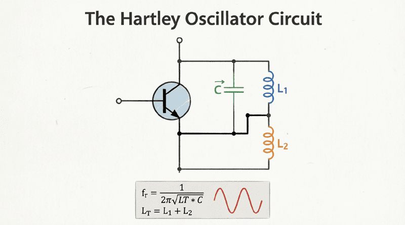
2. The Tank Circuit: The frequency-determining network, consisting of a single capacitor ($C$) connected in parallel with two series inductors ($L_1$ and $L_2$).
3. The Feedback Network: The center tap of the inductors is connected to the emitter (or source/ground) of the amplifier. This creates an inductive voltage divider that feeds a portion of the output signal back to the input.

The Phase Shift Mechanism

For any oscillator to work, it must satisfy the Barkhausen criterion, which requires a total loop phase shift of 0° (or 360°). The Hartley oscillator achieves this elegantly:

1. Amplifier Phase Shift: A common-emitter (or common-source) amplifier inherently introduces a 180° phase shift between its input (base/gate) and output (collector/drain).
2. Tank Circuit Phase Shift: The center tap of the inductor coil is connected to the AC ground (the emitter). Because the top and bottom ends of the coil are on opposite sides of this center tap, the voltage at the collector is exactly 180° out of phase with the voltage at the base.

Adding these together: 180° (amplifier) + 180° (tank circuit) = 360° (or 0°). This creates the positive (regenerative) feedback necessary to sustain oscillations.

Tapped Coil vs. Two Separate Inductors

In practical schematics, you will see the Hartley tank circuit drawn in two ways:

• Two Separate Inductors ($L_1$ and $L_2$): Easier to draw and analyze mathematically. They are placed in series, and their junction is tapped.
• A Single Tapped Inductor: In actual physical construction, a single coil of wire with a physical tap is often used. This is more compact and reduces parasitic resistance. If the two inductors are wound on the same core, mutual inductance ($M$) must be considered in the calculations.

How does the Hartley oscillator achieve the required 360-degree phase shift?
The common-emitter amplifier provides a 180-degree phase shift. The center-tapped inductor in the tank circuit provides the remaining 180-degree phase shift because the voltages at the two ends of the coil are opposite in polarity relative to the center tap (which is at AC ground).

Mathematical Analysis of the Hartley Oscillator

To design or analyze a Hartley oscillator, we must determine its frequency of oscillation and the required amplifier gain.

Frequency of Oscillation

The resonant frequency is determined by the total inductance of the tank circuit and the capacitance.

If we assume two separate inductors with no mutual coupling, the total inductance ($L_T$) is simply the sum of the two:

$L_T = L_1 + L_2$

The frequency of oscillation ($f_r$) is then given by the standard LC resonance formula:

$f_r = \frac{1}{2\pi\sqrt{L_T C}} = \frac{1}{2\pi\sqrt{(L_1 + L_2)C}}$

If Mutual Inductance Exists:
If $L_1$ and $L_2$ are wound on the same core (a single tapped coil), mutual inductance ($M$) affects the total inductance. Depending on the winding direction, the total inductance becomes:

$L_T = L_1 + L_2 \pm 2M$

(Usually, they are wound in the same direction, so it is $+2M$).

Feedback Fraction and Gain Requirement

The feedback fraction ($\beta$) is the ratio of the feedback voltage to the output voltage. In the Hartley oscillator, the feedback is taken from $L_2$ (the portion connected to the base), while the output is across $L_1$ (the portion connected to the collector).

Assuming negligible mutual inductance, the feedback fraction is proportional to the turns ratio or inductance ratio:

$\beta = \frac{V_{feedback}}{V_{output}} = \frac{L_2}{L_1}$

According to the Barkhausen criterion, the loop gain must be at least unity ($A_v \times \beta \geq 1$). Therefore, the minimum voltage gain ($A_v$) required from the amplifier to start and sustain oscillations is:

$A_v \geq \frac{1}{\beta} = \frac{L_1}{L_2}$

This simple relationship is a major advantage of the Hartley oscillator: by adjusting the ratio of $L_1$ to $L_2$, the designer can easily set the required gain and feedback level.

Advantages and Disadvantages

Like all circuit topologies, the Hartley oscillator has specific strengths and weaknesses compared to its counterparts, particularly the Colpitts oscillator.

Advantages

1. Easy Frequency Tuning: Because the frequency is determined by $C$ and $(L_1 + L_2)$, you can use a single variable capacitor to tune the frequency over a wide range without affecting the feedback ratio. This makes it the ideal choice for VFOs (Variable Frequency Oscillators) in radio receivers.
2. Simple Design: The circuit requires very few components and is straightforward to build on a breadboard or PCB.
3. Wide Frequency Range: It can operate from a few kilohertz up to several tens of megahertz, depending on the active device used.
4. Adjustable Feedback: The feedback level can be easily optimized by moving the tap on the inductor coil.

Disadvantages

1. Poor Waveform Purity: The Hartley oscillator tends to produce an output waveform with higher harmonic distortion compared to the Colpitts oscillator. The inductive feedback network is more susceptible to parasitic capacitances at high frequencies.
2. Frequency Stability: At very high frequencies (VHF and above), stray capacitances across the inductors can cause the frequency to drift or become unstable.
3. Bulky Inductors: For low-frequency operation, the required inductors can be physically large and heavy compared to the capacitors used in a Colpitts design.

What is the main advantage of a Hartley oscillator over a Colpitts oscillator?
The primary advantage of the Hartley oscillator is its ease of tuning. By using a single variable capacitor in the tank circuit, the frequency can be adjusted over a wide range without altering the feedback ratio, making it superior for Variable Frequency Oscillator (VFO) applications.

Practical Design Example

Let’s walk through the step-by-step design of a Hartley oscillator operating at 1 MHz using an NPN BJT transistor.

Step 1: Define Specifications

• Target Frequency ($f_r$): 1 MHz
• Supply Voltage ($V_{CC}$): 12V
• Transistor: 2N3904 (General purpose NPN, $f_T \approx 300$ MHz)

Step 2: Select the Capacitor

Choose a standard, stable capacitor value for the tank circuit. Let’s select:
$C = 100 \text{ pF}$ (100 × 10⁻¹² F)

Step 3: Calculate Total Inductance

Rearrange the frequency formula to solve for $L_T$:

$L_T = \frac{1}{(2\pi f_r)^2 C}$

$L_T = \frac{1}{(2\pi \times 1 \times 10^6)^2 \times 100 \times 10^{-12}}$

$L_T = \frac{1}{(6.283 \times 10^6)^2 \times 10^{-10}}$

$L_T = \frac{1}{3.947 \times 10^{13} \times 10^{-10}} = \frac{1}{3947}$

$L_T \approx 253.3 \text{ \mu H}$

Step 4: Split the Inductance ($L_1$ and $L_2$)

We need to divide $L_T$ into $L_1$ and $L_2$. A common rule of thumb for good startup and stable amplitude is to make $L_1$ roughly 2 to 3 times larger than $L_2$.

Let’s choose a ratio of roughly 3:1.
$L_1 = 190 \text{ \mu H}$
$L_2 = 63.3 \text{ \mu H}$

(Check: 190 + 63.3 = 253.3 \mu H. Perfect.)

Step 5: Determine Required Gain

Using the gain formula:

$A_v \geq \frac{L_1}{L_2} = \frac{190}{63.3} \approx 3.0$

The transistor amplifier must have a voltage gain of at least 3.0. In a common-emitter amplifier, gain is roughly $R_C / R_E$. Choosing $R_C = 3\text{k}\Omega$ and $R_E = 1\text{k}\Omega$ gives a theoretical gain of 3, which is sufficient to start oscillations. (In practice, the transistor’s non-linearities will limit the steady-state amplitude).

Step 6: Bias the Transistor

Design a standard voltage divider bias network for the 2N3904 to set the Q-point at roughly $V_{CE} = 6\text{V}$ and $I_C = 2\text{mA}$.

• $R_1$ (top base resistor) ≈ 56 kΩ
• $R_2$ (bottom base resistor) ≈ 10 kΩ
• Add an RF Choke (RFC) or a large resistor in the collector path if using a specific RF topology, though a standard resistive collector load works fine for basic 1 MHz designs.

Amplitude Stabilization

In the design example above, the initial loop gain is slightly greater than 3.0 to ensure oscillations start. However, if the gain remains at 3.0, the output amplitude would theoretically grow to infinity, which is impossible. In reality, the amplitude is limited by the non-linear characteristics of the active device.

As the oscillation amplitude increases, the transistor is driven into its saturation and cut-off regions during the peaks of the waveform. This “clipping” effectively reduces the average gain of the amplifier over a full cycle until the loop gain settles at exactly 1.0.

While this self-limiting mechanism is simple, it introduces harmonic distortion into the output waveform. For applications requiring a pure sine wave, an Automatic Level Control (ALC) circuit or a JFET used as a voltage-variable resistor in the feedback path can be implemented to smoothly reduce the gain without hard clipping.

Real-World Applications

1. Radio Receivers (Local Oscillators)

In superheterodyne AM radio receivers, the Hartley oscillator is frequently used as the local oscillator. The user turns the tuning knob, which rotates the plates of a variable capacitor in the Hartley tank circuit, sweeping the frequency to mix with incoming radio stations.

2. Signal Generators

Bench-top RF signal generators often utilize Hartley topologies in their lower frequency bands because the wide tuning range provided by a variable capacitor is highly desirable for sweeping frequencies.

3. Metal Detectors

Beat Frequency Oscillators (BFO) in metal detectors often use a Hartley configuration. The search coil itself acts as one of the inductors ($L_1$). When metal approaches the coil, the inductance changes, shifting the oscillator’s frequency and creating an audible beat note.

4. Educational and Hobbyist Projects

Because it requires only a few inexpensive components and clearly demonstrates the principles of inductive feedback, the Hartley oscillator is a standard project in university electronics labs and amateur radio (ham radio) building guides.

Summary and Conclusion

The Hartley oscillator is a classic, robust, and highly practical LC oscillator topology. By utilizing a tapped inductor to provide the necessary 180-degree phase shift for positive feedback, it simplifies the design of variable frequency oscillators and remains a vital tool in RF engineering.

Key Takeaways:

1. Topology: Uses a single capacitor and two series inductors (or a tapped coil) for the LC tank circuit.
2. Phase Shift: The common-emitter amplifier provides 180°, and the center-tapped inductor provides the remaining 180°, satisfying the Barkhausen criterion.
3. Frequency Formula: $f_r = \frac{1}{2\pi\sqrt{(L_1 + L_2)C}}$.
4. Feedback and Gain: The feedback fraction is $\beta = L_2 / L_1$, requiring a minimum amplifier gain of $A_v \geq L_1 / L_2$.
5. Primary Advantage: Excellent for VFO applications because frequency can be tuned with a single variable capacitor without affecting the feedback ratio.
6. Primary Disadvantage: Output waveform contains more harmonics than a Colpitts oscillator, and it is less stable at very high (VHF/UHF) frequencies.

Mastering the Hartley oscillator provides a deep understanding of inductive coupling and feedback networks. Whether you are tuning an AM radio, building a metal detector, or designing an RF signal source, the principles of the Hartley oscillator will serve as a foundational pillar in your electronics toolkit.