Armstrong Oscillator

Armstrong Oscillator: Complete Guide to Transformer-Coupled LC Oscillators

Introduction to the Armstrong Oscillator

The Armstrong Oscillator, also known as the Meissner Oscillator in European literature, holds a distinguished place in the history of radio technology. Invented by American engineer Edwin Howard Armstrong in 1912, this circuit was one of the first practical electronic oscillators and played a pivotal role in the development of radio communication.

Armstrong’s invention was revolutionary because it provided a reliable method for generating continuous radio frequency (RF) signals using a transformer-coupled feedback mechanism. Unlike earlier spark-gap transmitters that produced damped waves, the Armstrong oscillator generated continuous, undamped sinusoidal oscillations—essential for clear radio transmission and reception.

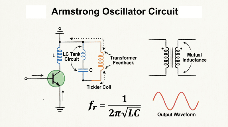
The defining characteristic of the Armstrong oscillator is its use of a tickler coil (a small feedback winding) magnetically coupled to the main LC tank circuit. This transformer coupling provides the necessary feedback to sustain oscillations while maintaining excellent isolation between the output and the frequency-determining network.

While modern solid-state oscillators have largely replaced the Armstrong topology in contemporary designs, understanding this circuit remains essential for:

• Appreciating the historical development of radio technology
• Understanding transformer-coupled feedback principles
• Designing high-isolation RF oscillators
• Troubleshooting vintage radio equipment

This comprehensive guide will explore the Armstrong oscillator’s unique topology, mathematical analysis, practical design considerations, and its enduring legacy in RF engineering.

What is an Armstrong Oscillator?
An Armstrong oscillator is an LC oscillator circuit that uses transformer coupling (a tickler coil) to provide feedback from the output to the input. The tickler coil is magnetically coupled to the main LC tank circuit, providing the necessary phase shift and feedback to sustain oscillations. It was one of the first practical RF oscillators, invented by Edwin Armstrong in 1912.

Circuit Topology and Operation

The Basic Configuration

The Armstrong oscillator consists of three fundamental components:

1. The Amplifier: Typically a vacuum tube (in historical designs) or a transistor (BJT or FET) in modern implementations. The amplifier is configured in a common-emitter (or common-source/common-cathode) configuration.
2. The LC Tank Circuit: A parallel resonant circuit consisting of an inductor ($L$) and capacitor ($C$) that determines the frequency of oscillation. This is the main frequency-determining network.
3. The Tickler Coil (Feedback Winding): A small inductor ($L_f$) magnetically coupled to the main tank inductor. This coil provides the feedback signal necessary to sustain oscillations.

Transformer Coupling and Feedback

The key to the Armstrong oscillator’s operation is the mutual inductance between the tickler coil and the main tank inductor. This coupling is characterized by the coupling coefficient ($k$), which ranges from 0 (no coupling) to 1 (perfect coupling).

How Feedback Works:

1. Signal Generation: Random noise or power-on transients initiate oscillations in the LC tank circuit.
2. Magnetic Coupling: The oscillating current in the tank inductor creates a varying magnetic field.
3. Induced Voltage: This magnetic field induces a voltage in the tickler coil according to Faraday’s law of induction.
4. Feedback: The induced voltage is fed back to the amplifier input (base/gate).
5. Amplification: The amplifier amplifies this signal and feeds it back to the tank circuit, sustaining the oscillations.

Phase Shift and Polarity

For sustained oscillations, the feedback must be positive (regenerative), meaning it must reinforce the original signal. This requires:

1. Amplifier Phase Shift: The common-emitter amplifier provides 180° phase shift.
2. Transformer Phase Shift: The transformer must provide an additional 180° phase shift. This is achieved by proper winding polarity (dot convention).

If the tickler coil is wound in the wrong direction, the feedback will be negative (degenerative), and the circuit will not oscillate.

Dot Convention:

• If the dot on the tank inductor is at the collector side, the dot on the tickler coil should be at the base side (for NPN transistor).
• This ensures the feedback signal is in phase with the original signal after the 180° amplifier inversion.

What is a tickler coil?
A tickler coil is a small feedback winding in an Armstrong oscillator that is magnetically coupled to the main LC tank inductor. It picks up a portion of the oscillating signal through mutual inductance and feeds it back to the amplifier input to sustain oscillations. The name “tickler” comes from its function of “tickling” the input to keep oscillations going.

Mathematical Analysis of the Armstrong Oscillator

Frequency of Oscillation

The frequency of oscillation is primarily determined by the LC tank circuit:

$f_r = \frac{1}{2\pi\sqrt{LC}}$

Where:

• $f_r$ = Frequency of oscillation in Hertz (Hz)
• $L$ = Inductance of the main tank coil in Henrys (H)
• $C$ = Capacitance in Farads (F)

In practice, the actual frequency may be slightly different due to:

• Stray capacitances in the circuit
• Loading effects from the amplifier
• Mutual inductance effects
• Component tolerances

Mutual Inductance and Coupling

The mutual inductance ($M$) between the tickler coil and the tank inductor is:

$M = k\sqrt{L \times L_f}$

Where:

• $k$ = Coupling coefficient (0 < k < 1)
• $L$ = Inductance of the main tank coil
• $L_f$ = Inductance of the tickler coil

Typical coupling coefficients for Armstrong oscillators range from 0.1 to 0.5 (loose coupling).

Gain Requirement

For oscillations to start and be sustained, the loop gain must satisfy the Barkhausen criterion:

$A_v \times \beta \geq 1$

Where:

• $A_v$ = Voltage gain of the amplifier
• $\beta$ = Feedback factor

The feedback factor in an Armstrong oscillator is approximately:

$\beta \approx \frac{M}{L} = k\sqrt{\frac{L_f}{L}}$

Therefore, the minimum gain required is:

$A_v \geq \frac{1}{\beta} = \frac{1}{k}\sqrt{\frac{L}{L_f}}$

This shows that:

• Tighter coupling (higher k) requires less gain
• A smaller tickler coil (lower $L_f$) requires more gain
• There’s a trade-off between coupling strength and gain requirements

Optimal Coupling

If the coupling is too loose (k too small):

• Insufficient feedback
• Oscillations may not start or may be weak
• Frequency stability is poor

If the coupling is too tight (k too large):

• Excessive feedback
• Waveform distortion (clipping)
• Frequency pulling (tank circuit loaded by amplifier)
• Reduced frequency stability

Optimal range: k = 0.2 to 0.3 for most applications.

Practical Design Example: 1 MHz Armstrong Oscillator

Let’s design a practical Armstrong oscillator operating at 1 MHz using a 2N3904 NPN transistor.

Step 1: Define Specifications

• Target Frequency ($f_r$): 1.0 MHz
• Supply Voltage ($V_{CC}$): 12V
• Transistor: 2N3904 (General purpose NPN, $f_T \approx 300$ MHz)
• Coupling Coefficient (k): 0.25 (typical)

Step 2: Select the Tank Capacitor

Choose a practical capacitor value for 1 MHz operation.

$C = 100 \text{ pF}$ ($100 \times 10^{-12}$ F)

Step 3: Calculate the Tank Inductor

Rearrange the frequency formula to solve for $L$:

$L = \frac{1}{(2\pi f_r)^2 C}$

$L = \frac{1}{(2\pi \times 1 \times 10^6)^2 \times 100 \times 10^{-12}}$

$L = \frac{1}{(6.283 \times 10^6)^2 \times 10^{-10}}$

$L = \frac{1}{3.947 \times 10^{13} \times 10^{-10}}$

$L = \frac{1}{3947} \approx 253 \times 10^{-6}$

$L \approx 250 \text{ μH}$ (use standard value)

Step 4: Calculate Tickler Coil Inductance

For good feedback without excessive loading, the tickler coil should have an inductance of approximately 1/10 to 1/4 of the main tank inductance.

Let’s choose:
$L_f = \frac{L}{4} = \frac{250 \text{ μH}}{4} = 62.5 \text{ μH}$

Use standard value: $L_f = 68 \text{ μH}$

Step 5: Verify Coupling and Gain

With k = 0.25:

Mutual inductance:
$M = k\sqrt{L \times L_f} = 0.25\sqrt{250 \times 68} = 0.25\sqrt{17000} = 0.25 \times 130.4 = 32.6 \text{ μH}$

Feedback factor:
$\beta \approx \frac{M}{L} = \frac{32.6}{250} = 0.13$

Minimum gain required:
$A_v \geq \frac{1}{\beta} = \frac{1}{0.13} \approx 7.7$

A common-emitter amplifier with proper biasing can easily provide a gain of 10-50, so this design should work well.

Step 6: Bias Network Design

Design a standard voltage divider bias for the 2N3904:

• Target $I_C = 2 \text{ mA}$
• Target $V_{CE} = 6 \text{ V}$ (mid-supply)
• $R_C = 2.2 \text{ k}\Omega$
• $R_E = 1 \text{ k}\Omega$ (bypassed with 10 μF capacitor for AC gain)
• $R_1 = 47 \text{ k}\Omega$
• $R_2 = 10 \text{ k}\Omega$

Step 7: Physical Construction

Wind the tank coil and tickler coil on the same form:

• Use a ferrite rod or air-core form
• Wind the main coil (250 μH) first
• Wind the tickler coil (68 μH) over or adjacent to the main coil
• Ensure proper phasing (dot convention)
• Adjust spacing to achieve k ≈ 0.25

Advantages and Disadvantages

Advantages

1. Excellent Isolation: The transformer coupling provides excellent isolation between the output and the frequency-determining tank circuit. This minimizes frequency pulling due to load variations.
2. Good Frequency Stability: The high-Q tank circuit is not directly loaded by the amplifier, resulting in better frequency stability compared to directly-coupled oscillators.
3. Simple Design: The circuit is relatively simple to understand and build, requiring only a few components.
4. Adjustable Feedback: The coupling coefficient can be adjusted by changing the physical spacing or orientation of the coils, allowing fine-tuning of the feedback level.
5. Historical Significance: Understanding this circuit provides insight into the development of radio technology and oscillator theory.

Disadvantages

1. Bulky Components: The transformer (two coupled inductors) is physically larger and heavier than the capacitive or inductive dividers used in other oscillator types.
2. Difficult to Integrate: The transformer coupling makes it difficult to implement in integrated circuits (ICs), limiting its use in modern miniaturized electronics.
3. Critical Phasing: The winding polarity must be correct for oscillation to occur. Reversing the tickler coil connections will prevent oscillation.
4. Limited Frequency Range: While suitable for RF applications, the Armstrong oscillator is less practical at very high frequencies (VHF/UHF) due to transformer parasitics and at very low frequencies due to the large inductors required.
5. Component Availability: Custom-wound transformers or coupled inductors may be difficult to source compared to standard capacitors and resistors.

Why is the Armstrong oscillator less common in modern designs?
The Armstrong oscillator requires a transformer (coupled inductors) for feedback, which is bulky, expensive, and difficult to integrate into modern ICs. Modern oscillators like the Colpitts and Hartley use capacitive or tapped-inductive feedback that is easier to miniaturize and integrate, making them more suitable for contemporary electronics.

Real-World Applications

1. Historical Radio Transmitters

The Armstrong oscillator was widely used in early radio transmitters from the 1920s to 1950s. Its ability to generate stable, continuous RF signals made it ideal for AM broadcasting.

2. Vintage Radio Receivers

Many vintage radio receivers used Armstrong oscillators as local oscillators in superheterodyne circuits. These radios are still collected and restored by hobbyists today.

3. Educational Demonstrations

The Armstrong oscillator is an excellent teaching tool for demonstrating:

• Transformer coupling principles
• Mutual inductance
• Feedback theory
• Oscillator operation
• Radio frequency generation

4. High-Isolation RF Oscillators

In applications where excellent isolation between the oscillator and load is critical, the Armstrong topology may still be preferred over modern alternatives.

5. Low-Frequency Signal Generation

With appropriate component values, Armstrong oscillators can generate low-frequency signals for test and measurement applications.

Comparison with Other LC Oscillators

Feature	Armstrong	Hartley	Colpitts
Feedback Method	Transformer (tickler coil)	Tapped inductor	Tapped capacitor
Isolation	Excellent	Good	Fair
Component Count	Moderate	Low	Low
Size/Weight	Large (transformer)	Moderate	Small
IC Compatibility	Poor	Moderate	Good
Frequency Stability	Good	Good	Excellent
Ease of Tuning	Moderate	Good	Good
Historical Significance	Very High	High	High

Summary: The Armstrong oscillator excels in isolation and frequency stability but suffers from size and integration limitations. Modern designs typically prefer Hartley or Colpitts topologies for their compactness and IC compatibility.

The Armstrong oscillator represents a landmark achievement in the history of electronics. Edwin Armstrong’s ingenious use of transformer coupling to provide feedback laid the foundation for modern RF oscillator design and enabled the development of practical radio communication systems.

Key Takeaways:

1. Topology: Uses a tickler coil (feedback winding) magnetically coupled to the main LC tank circuit to provide regenerative feedback.
2. Frequency Formula: $f_r = \frac{1}{2\pi\sqrt{LC}}$ (determined by the tank circuit).
3. Mutual Inductance: $M = k\sqrt{L \times L_f}$, where k is the coupling coefficient (typically 0.2-0.3).
4. Gain Requirement: $A_v \geq \frac{1}{k}\sqrt{\frac{L}{L_f}}$
5. Primary Advantages:

• Excellent isolation between output and tank circuit
• Good frequency stability
• Simple design principle
• Adjustable feedback via coupling

6. Primary Disadvantages:

• Bulky transformer components
• Poor IC compatibility
• Critical winding polarity
• Limited modern applications

7. Historical Legacy: The Armstrong oscillator was instrumental in the development of radio technology and remains an important educational tool for understanding oscillator principles.

While the Armstrong oscillator has been largely superseded by more compact and integrable designs in modern electronics, its principles remain fundamental to understanding feedback, transformer coupling, and oscillator operation. For hobbyists, historians, and students of electronics, the Armstrong oscillator offers a tangible connection to the pioneering days of radio and a deep appreciation for the ingenuity of early electronic engineers.